
BIG DATA ANALYTICS
[R17A0528]
LECTURE NOTES
B.TECH IV YEAR – I SEM (R17)
(2020-2021)
MALLA REDDY
COLLEGE OF ENGINEERING & TECHNOLOGY
(Autonomous Institution – UGC, Govt. of India)
Recognized under 2(f) and 12 (B) of UGC ACT 1956
(Affiliated to JNTUH, Hyderabad, Approved by AICTE - Accredited by NBA & NAAC – ‘A’ Grade - ISO 9001:2015 Certified)
Maisammaguda, Dhulapally (Post Via. Hakimpet), Secunderabad – 500100, Telangana State, India
(R17A0528) BIG DATA ANALYTICS
UNIT I
INTRODUCTION TO BIG DATA AND ANALYTICS
Classification of Digital Data, Structured and Unstructured Data –
Introduction to Big Data: Characteristics – Evolution – Definition - Challenges with Big Data
- Other Characteristics of Data - Why Big Data - Traditional Business Intelligence versus Big
Data - Data Warehouse and Hadoop Environment Big Data Analytics: Classification of
Analytics – Challenges - Big Data Analytics important - Data Science - Data Scientist -
Terminologies used in Big Data Environments - Basically Available Soft State Eventual
Consistency - Top Analytics Tools
UNIT II
INTRODUCTION TO TECHNOLOGY LANDSCAPE
NoSQL, Comparison of SQL and NoSQL, Hadoop -RDBMS Versus Hadoop - Distributed
Computing Challenges – Hadoop Overview - Hadoop Distributed File System - Processing
Data with Hadoop - Managing Resources and Applications with Hadoop YARN -
Interacting with Hadoop Ecosystem
UNIT III
INTRODUCTION TO MONGODB AND MAPREDUCE PROGRAMMING
MongoDB: Why Mongo DB - Terms used in RDBMS and Mongo DB - Data Types -
MongoDB Query Language
MapReduce: Mapper – Reducer – Combiner – Partitioner – Searching – Sorting – Compression
UNIT IV
INTRODUCTION TO HIVE AND PIG
Hive: Introduction – Architecture - Data Types - File Formats - Hive Query Language
Statements – Partitions – Bucketing – Views - Sub- Query – Joins – Aggregations - Group by
and Having - RCFile Implementation - Hive User Defined Function - Serialization and
Deserialization. Pig: Introduction - Anatomy – Features – Philosophy - Use Case for Pig - Pig
Latin Overview - Pig Primitive Data Types - Running Pig - Execution Modes of Pig - HDFS
Commands - Relational Operators - Eval Function - Complex Data Types - Piggy Bank -
User-Defined Functions - Parameter Substitution - Diagnostic Operator - Word Count
Example using Pig - Pig at Yahoo! - Pig Versus Hive
UNIT V
INTRODUCTION TO DATA ANALYTICS WITH R
Machine Learning: Introduction, Supervised Learning, Unsupervised Learning, Machine
Learning Algorithms: Regression Model, Clustering, Collaborative Filtering, Associate Rule
Making, Decision Tree, Big Data Analytics with BigR.
Reference Book:
1. Judith Huruwitz, Alan Nugent, Fern Halper, Marcia Kaufman, “Big data for
dummies”, John Wiley & Sons, Inc.(2013)
2. Tom White, “Hadoop The Definitive Guide”, O’Reilly Publications, Fourth
Edition,2015
3. Dirk Deroos, Paul C.Zikopoulos, Roman B.Melnky, Bruce Brown, Rafael Coss,
“Hadoop For Dummies”, Wiley Publications,2014
4. Robert D.Schneider, “Hadoop For Dummies”, John Wiley & Sons, Inc.(2012)
5. Paul Zikopoulos, “Understanding Big Data: Analytics for Enterprise Class
Hadoop and Streaming Data, McGraw Hill, 2012 Chuck Lam, “Hadoop In
Action”, Dreamtech Publications, 2010
Text Book:
1. Seema Acharya, Subhashini Chellappan, “Big Data and Analytics”, Wiley
Publications, First Edition,2015

INDEX
S. No
Unit
Topic
Pg.No
1
I
INTRODUCTION TO BIG DATA AND ANALYTICS
Classification of Digital Data, Structured and Unstructured Data -
Introduction to Big Data
1
2
I
Why Big Data Traditional Business Intelligence versus Big Data - Data
Warehouse and Hadoop
4
3
I
Environment Big Data Analytics: Classification of Analytics – Challenges
- Big Data Analytics importance
5
4
I
Data Science - Data Scientist - Terminologies used in Big Data Environments
10
5
I
Basically, Available Soft State Eventual Consistency -Top Analytics Tools
12
7
II
INTRODUCTION TO TECHNOLOGY LANDSCAPE
NoSQL, Comparison of SQL and NoSQL, Hadoop -RDBMS Versus
Hadoop - Distributed Computing
15
8
II
Challenges – Hadoop Overview - Hadoop Distributed File System -
Processing Data with Hadoop -
20
9
II
Managing Resources and Applications with Hadoop YARN -
Interacting with Hadoop Ecosystem
22
111
10
III
INTRODUCTION TO MONGODB AND MAPREDUCE
PROGRAMMING
MongoDB: Why Mongo DB - Terms used in RDBMS and Mongo DB -
Data Types - MongoDB Query Language
24
1
11
III
MapReduce: Mapper – Reducer – Combiner – Partitioner – Searching –
Sorting – Compression
36
12
IV
INTRODUCTION TO HIVE AND PIG
Hive: Introduction – Architecture - Data Types - File Formats - Hive
Query Language Statements
52
13
IV
Partitions – Bucketing – Views - Sub- Query – Joins – Aggregations -
Group by and Having - RCFile
70
14
IV
Implementation – Hive User Defined Function - Serialization and
Deserialization. Pig: Introduction
75
15
IV
Anatomy – Features – Philosophy - Use Case for Pig - Pig Latin
Overview - Pig Primitive Data Types
76
16
IV
Running Pig - Execution Modes of Pig - HDFS Commands -Relational
Operators - Eval Function
79
17
IV
Complex Data Types - Piggy Bank - User-Defined Functions -
Parameter Substitution – Diagnostic
82
18
IV
Operator - Word Count Example using Pig - Pig at Yahoo! - Pig Versus
Hive
93
19
V
INTRODUCTION TO DATA ANALYTICS WITH R
Machine Learning: Introduction, Supervised Learning, Unsupervised
Learning, Machine Learning
96
20
V
Algorithms: Regression Model, Clustering, Collaborative Filtering,
Associate Rule Making, Decision Tree, Big Data Analytics with BigR.
97

BIG DATA ANALYTICS
1
UNIT – I
What is Big Data?
According to Gartner, the definition of Big Data –
“Big data” is high-volume, velocity, and variety information assets that demand cost-effective,
innovative forms of information processing for enhanced insight and decision making.”
This definition clearly answers the “What is Big Data?” question – Big Data refers to complex and
large data sets that have to be processed and analyzed to uncover valuable information that can
benefit businesses and organizations.
However, there are certain basic tenets of Big Data that will make it even simpler to answer what
is Big Data:
It refers to a massive amount of data that keeps on growing exponentially with time.
It is so voluminous that it cannot be processed or analyzed using conventional data
processing techniques.
It includes data mining, data storage, data analysis, data sharing, and data visualization.
The term is an all-comprehensive one including data, data frameworks, along with the tools
and techniques used to process and analyze the data.
The History of Big Data
Although the concept of big data itself is relatively new, the origins of large data sets go back to
the 1960s and '70s when the world of data was just getting started with the first data centers and
the development of the relational database.
Around 2005, people began to realize just how much data users generated through Facebook,
YouTube, and other online services. Hadoop (an open-source framework created specifically to
store and analyze big data sets) was developed that same year. NoSQL also began to gain
popularity during this time.
The development of open-source frameworks, such as Hadoop (and more recently, Spark) was
essential for the growth of big data because they make big data easier to work with and cheaper to
store. In the years since then, the volume of big data has skyrocketed. Users are still generating
huge amounts of data—but it’s not just humans who are doing it.
With the advent of the Internet of Things (IoT), more objects and devices are connected to the
internet, gathering data on customer usage patterns and product performance. The emergence of
machine learning has produced still more data.
While big data has come far, its usefulness is only just beginning. Cloud computing has expanded
big data possibilities even further. The cloud offers truly elastic scalability, where developers can
simply spin up ad hoc clusters to test a subset of data.

BIG DATA ANALYTICS
2
Benefits of Big Data and Data Analytics
Big data makes it possible for you to gain more complete answers because you have more
information.
More complete answers mean more confidence in the data—which means a completely
different approach to tackling problems.
Types of Big Data
Now that we are on track with what is big data, let’s have a look at the types of big data:
a) Structured
Structured is one of the types of big data and By structured data, we mean data that can be
processed, stored, and retrieved in a fixed format. It refers to highly organized information that
can be readily and seamlessly stored and accessed from a database by simple search engine
algorithms. For instance, the employee table in a company database will be structured as the
employee details, their job positions, their salaries, etc., will be present in an organized manner.
b) Unstructured
Unstructured data refers to the data that lacks any specific form or structure whatsoever. This
makes it very difficult and time-consuming to process and analyze unstructured data. Email is an
example of unstructured data. Structured and unstructured are two important types of big data.
c) Semi-structured
Semi structured is the third type of big data. Semi-structured data pertains to the data containing
both the formats mentioned above, that is, structured and unstructured data. To be precise, it refers
to the data that although has not been classified under a particular repository (database), yet
contains vital information or tags that segregate individual elements within the data. Thus we come
to the end of types of data.
Characteristics of Big Data
Back in 2001, Gartner analyst Doug Laney listed the 3 ‘V’s of Big Data – Variety, Velocity, and
Volume. Let’s discuss the characteristics of big data.
These characteristics, isolated, are enough to know what big data is. Let’s look at them in depth:
a) Variety
Variety of Big Data refers to structured, unstructured, and semi-structured data that is gathered
from multiple sources. While in the past, data could only be collected from spreadsheets and
databases, today data comes in an array of forms such as emails, PDFs, photos, videos, audios, SM
posts, and so much more. Variety is one of the important characteristics of big data.

BIG DATA ANALYTICS
3
b) Velocity
Velocity essentially refers to the speed at which data is being created in real-time. In a broader
prospect, it comprises the rate of change, linking of incoming data sets at varying speeds, and
activity bursts.
c) Volume
Volume is one of the characteristics of big data. We already know that Big Data indicates huge
‘volumes’ of data that is being generated on a daily basis from various sources like social media
platforms, business processes, machines, networks, human interactions, etc. Such a large amount
of data is stored in data warehouses. Thus comes to the end of characteristics of big data.
Why is Big Data Important?
The importance of big data does not revolve around how much data a company has but how a
company utilizes the collected data. Every company uses data in its own way; the more efficiently
a company uses its data, the more potential it has to grow. The company can take data from any
source and analyze it to find answers which will enable:
1. Cost Savings: Some tools of Big Data like Hadoop and Cloud-Based Analytics can
bring cost advantages to business when large amounts of data are to be stored and these
tools also help in identifying more efficient ways of doing business.
2. Time Reductions: The high speed of tools like Hadoop and in-memory analytics can
easily identify new sources of data which helps businesses analyzing data immediately
and make quick decisions based on the learning.
3. Understand the market conditions: By analyzing big data you can get a better
understanding of current market conditions. For example, by analyzing customers’
purchasing behaviors, a company can find out the products that are sold the most and
produce products according to this trend. By this, it can get ahead of its competitors.
4. Control online reputation: Big data tools can do sentiment analysis. Therefore, you
can get feedback about who is saying what about your company. If you want to monitor
and improve the online presence of your business, then, big data tools can help in all
this.
5. Using Big Data Analytics to Boost Customer Acquisition and Retention
The customer is the most important asset any business depends on. There is no single
business that can claim success without first having to establish a solid customer base.
However, even with a customer base, a business cannot afford to disregard the high
competition it faces. If a business is slow to learn what customers are looking for, then
it is very easy to begin offering poor quality products. In the end, loss of clientele will
result, and this creates an adverse overall effect on business success. The use of big data
allows businesses to observe various customer related patterns and trends. Observing
customer behavior is important to trigger loyalty.
6. Using Big Data Analytics to Solve Advertisers Problem and Offer Marketing
Insights

BIG DATA ANALYTICS
4
Big data analytics can help change all business operations. This includes the ability to
match customer expectation, changing company’s product line and of course ensuring
that the marketing campaigns are powerful.
7. Big Data Analytics As a Driver of Innovations and Product Development
Another huge advantage of big data is the ability to help companies innovate and
redevelop their products.
Business Intelligence vs Big Data
Although Big Data and Business Intelligence are two technologies used to analyze data to help
companies in the decision-making process, there are differences between both of them. They differ
in the way they work as much as in the type of data they analyze.
Traditional BI methodology is based on the principle of grouping all business data into a central
server. Typically, this data is analyzed in offline mode, after storing the information in an
environment called Data Warehouse. The data is structured in a conventional relational database
with an additional set of indexes and forms of access to the tables (multidimensional cubes).
A Big Data solution differs in many aspects to BI to use. These are the main differences between
Big Data and Business Intelligence:
1. In a Big Data environment, information is stored on a distributed file system, rather than
on a central server. It is a much safer and more flexible space.
2. Big Data solutions carry the processing functions to the data, rather than the data to the
functions. As the analysis is centered on the information, it´s easier to handle larger
amounts of information in a more agile way.
3. Big Data can analyze data in different formats, both structured and unstructured. The
volume of unstructured data (those not stored in a traditional database) is growing at levels
much higher than the structured data. Nevertheless, its analysis carries different challenges.
Big Data solutions solve them by allowing a global analysis of various sources of
information.
4. Data processed by Big Data solutions can be historical or come from real-time sources.
Thus, companies can make decisions that affect their business in an agile and efficient way.
5. Big Data technology uses parallel mass processing (MPP) concepts, which improves the
speed of analysis. With MPP many instructions are executed simultaneously, and since the
various jobs are divided into several parallel execution parts, at the end the overall results
are reunited and presented. This allows you to analyze large volumes of information
quickly.

BIG DATA ANALYTICS
5
Big Data vs Data Warehouse
Big Data has become the reality of doing business for organizations today. There is a boom in the
amount of structured as well as raw data that floods every organization daily. If this data is
managed well, it can lead to powerful insights and quality decision making.
Big data analytics is the process of examining large data sets containing a variety of data types to
discover some knowledge in databases, to identify interesting patterns and establish relationships
to solve problems, market trends, customer preferences, and other useful information. Companies
and businesses that implement Big Data Analytics often reap several business benefits. Companies
implement Big Data Analytics because they want to make more informed business decisions.
A data warehouse (DW) is a collection of corporate information and data derived from operational
systems and external data sources. A data warehouse is designed to support business decisions by
allowing data consolidation, analysis and reporting at different aggregate levels. Data is populated
into the Data Warehouse through the processes of extraction, transformation and loading (ETL
tools). Data analysis tools, such as business intelligence software, access the data within the
warehouse.
Hadoop Environment Big Data Analytics
Hadoop is changing the perception of handling Big Data especially the unstructured data. Let’s
know how Apache Hadoop software library, which is a framework, plays a vital role in handling
Big Data. Apache Hadoop enables surplus data to be streamlined for any distributed processing
system across clusters of computers using simple programming models. It truly is made to scale
up from single servers to a large number of machines, each and every offering local computation,
and storage space. Instead of depending on hardware to provide high-availability, the library itself
is built to detect and handle breakdowns at the application layer, so providing an extremely
available service along with a cluster of computers, as both versions might be vulnerable to
failures.
Hadoop Community Package Consists of
File system and OS level abstractions
A MapReduce engine (either MapReduce or YARN)
The Hadoop Distributed File System (HDFS)
Java ARchive (JAR) files
Scripts needed to start Hadoop
Source code, documentation and a contribution section
Activities performed on Big Data

BIG DATA ANALYTICS
6
Store – Big data need to be collected in a seamless repository, and it is not necessary to
store in a single physical database.
Process – The process becomes more tedious than traditional one in terms of cleansing,
enriching, calculating, transforming, and running algorithms.
Access – There is no business sense of it at all when the data cannot be searched, retrieved
easily, and can be virtually showcased along the business lines.
Classification of analytics
Descriptive analytics
Descriptive analytics is a statistical method that is used to search and summarize historical data in
order to identify patterns or meaning.
Data aggregation and data mining are two techniques used in descriptive analytics to discover
historical data. Data is first gathered and sorted by data aggregation in order to make the datasets
more manageable by analysts.
Data mining describes the next step of the analysis and involves a search of the data to identify
patterns and meaning. Identified patterns are analyzed to discover the specific ways that learners
interacted with the learning content and within the learning environment.
Advantages:
Quickly and easily report on the Return on Investment (ROI) by showing how performance
achieved business or target goals.
Identify gaps and performance issues early - before they become problems.
Identify specific learners who require additional support, regardless of how many students
or employees there are.
Identify successful learners in order to offer positive feedback or additional resources.
Analyze the value and impact of course design and learning resources.
Predictive analytics
Predictive Analytics is a statistical method that utilizes algorithms and machine learning to identify
trends in data and predict future behaviors
The software for predictive analytics has moved beyond the realm of statisticians and is becoming
more affordable and accessible for different markets and industries, including the field of learning
& development.

BIG DATA ANALYTICS
7
For online learning specifically, predictive analytics is often found incorporated in the Learning
Management System (LMS), but can also be purchased separately as specialized software.
For the learner, predictive forecasting could be as simple as a dashboard located on the main screen
after logging in to access a course. Analyzing data from past and current progress, visual indicators
in the dashboard could be provided to signal whether the employee was on track with training
requirements.
Advantages:
Personalize the training needs of employees by identifying their gaps, strengths, and
weaknesses; specific learning resources and training can be offered to support individual
needs.
Retain Talent by tracking and understanding employee career progression and forecasting
what skills and learning resources would best benefit their career paths. Knowing what skills
employees need also benefits the design of future training.
Support employees who may be falling behind or not reaching their potential by offering
intervention support before their performance puts them at risk.
Simplified reporting and visuals that keep everyone updated when predictive forecasting
is required.
Prescriptive analytics
Prescriptive analytics is a statistical method used to generate recommendations and make decisions
based on the computational findings of algorithmic models.
Generating automated decisions or recommendations requires specific and unique algorithmic
models and clear direction from those utilizing the analytical technique. A recommendation cannot
be generated without knowing what to look for or what problem is desired to be solved. In this
way, prescriptive analytics begins with a problem.
Example
A Training Manager uses predictive analysis to discover that most learners without a particular
skill will not complete the newly launched course. What could be done? Now prescriptive analytics
can be of assistance on the matter and help determine options for action. Perhaps an algorithm can
detect the learners who require that new course, but lack that particular skill, and send an automated
recommendation that they take an additional training resource to acquire the missing skill.

BIG DATA ANALYTICS
8
The accuracy of a generated decision or recommendation, however, is only as good as the quality
of data and the algorithmic models developed. What may work for one company’s training needs
may not make sense when put into practice in another company’s training department. Models are
generally recommended to be tailored for each unique situation and need.
Descriptive vs Predictive vs Prescriptive Analytics
Descriptive Analytics is focused solely on historical data.
You can think of Predictive Analytics as then using this historical data to develop statistical models
that will then forecast about future possibilities.
Prescriptive Analytics takes Predictive Analytics a step further and takes the possible forecasted
outcomes and predicts consequences for these outcomes.
What Big Data Analytics Challenges
1. Need For Synchronization Across Disparate Data Sources
As data sets are becoming bigger and more diverse, there is a big challenge to incorporate them
into an analytical platform. If this is overlooked, it will create gaps and lead to wrong messages
and insights.
2. Acute Shortage Of Professionals Who Understand Big Data Analysis
The analysis of data is important to make this voluminous amount of data being produced in every
minute, useful. With the exponential rise of data, a huge demand for big data scientists and Big
Data analysts has been created in the market. It is important for business organizations to hire a
data scientist having skills that are varied as the job of a data scientist is multidisciplinary. Another
major challenge faced by businesses is the shortage of professionals who understand Big Data
analysis. There is a sharp shortage of data scientists in comparison to the massive amount of data
being produced.
3. Getting Meaningful Insights Through The Use Of Big Data Analytics
It is imperative for business organizations to gain important insights from Big Data analytics, and
also it is important that only the relevant department has access to this information. A big challenge
faced by the companies in the Big Data analytics is mending this wide gap in an effective manner.

BIG DATA ANALYTICS
9
4. Getting Voluminous Data Into The Big Data Platform
It is hardly surprising that data is growing with every passing day. This simply indicates that
business organizations need to handle a large amount of data on daily basis. The amount and
variety of data available these days can overwhelm any data engineer and that is why it is
considered vital to make data accessibility easy and convenient for brand owners and managers.
5. Uncertainty Of Data Management Landscape
With the rise of Big Data, new technologies and companies are being developed every day.
However, a big challenge faced by the companies in the Big Data analytics is to find out which
technology will be best suited to them without the introduction of new problems and potential
risks.
6. Data Storage And Quality
Business organizations are growing at a rapid pace. With the tremendous growth of the companies
and large business organizations, increases the amount of data produced. The storage of this
massive amount of data is becoming a real challenge for everyone. Popular data storage options
like data lakes/ warehouses are commonly used to gather and store large quantities of unstructured
and structured data in its native format. The real problem arises when a data lakes/ warehouse try
to combine unstructured and inconsistent data from diverse sources, it encounters errors. Missing
data, inconsistent data, logic conflicts, and duplicates data all result in data quality challenges.
7. Security And Privacy Of Data
Once business enterprises discover how to use Big Data, it brings them a wide range of possibilities
and opportunities. However, it also involves the potential risks associated with big data when it
comes to the privacy and the security of the data. The Big Data tools used for analysis and storage
utilizes the data disparate sources. This eventually leads to a high risk of exposure of the data,
making it vulnerable. Thus, the rise of voluminous amount of data increases privacy and security
concerns.
Terminologies Used In Big Data Environments
As-a-service infrastructure
Data-as-a-service, software-as-a-service, platform-as-a-service – all refer to the idea that rather
than selling data, licences to use data, or platforms for running Big Data technology, it can be
provided “as a service”, rather than as a product. This reduces the upfront capital investment

BIG DATA ANALYTICS
10
necessary for customers to begin putting their data, or platforms, to work for them, as the provider
bears all of the costs of setting up and hosting the infrastructure. As a customer, as-a-service
infrastructure can greatly reduce the initial cost and setup time of getting Big Data initiatives up
and running.
Data science
Data science is the professional field that deals with turning data into value such as new insights
or predictive models. It brings together expertise from fields including statistics, mathematics,
computer science, communication as well as domain expertise such as business knowledge. Data
scientist has recently been voted the No 1 job in the U.S., based on current demand and salary and
career opportunities.
Data mining
Data mining is the process of discovering insights from data. In terms of Big Data, because it is so
large, this is generally done by computational methods in an automated way using methods such
as decision trees, clustering analysis and, most recently, machine learning. This can be thought of
as using the brute mathematical power of computers to spot patterns in data which would not be
visible to the human eye due to the complexity of the dataset.
Hadoop
Hadoop is a framework for Big Data computing which has been released into the public domain
as open source software, and so can freely be used by anyone. It consists of a number of modules
all tailored for a different vital step of the Big Data process – from file storage (Hadoop File System
– HDFS) to database (HBase) to carrying out data operations (Hadoop MapReduce – see below).
It has become so popular due to its power and flexibility that it has developed its own industry of
retailers (selling tailored versions), support service providers and consultants.
Predictive modelling
At its simplest, this is predicting what will happen next based on data about what has happened
previously. In the Big Data age, because there is more data around than ever before, predictions
are becoming more and more accurate. Predictive modelling is a core component of most Big Data
initiatives, which are formulated to help us choose the course of action which will lead to the most
desirable outcome. The speed of modern computers and the volume of data available means that
predictions can be made based on a huge number of variables, allowing an ever-increasing number
of variables to be assessed for the probability that it will lead to success.
MapReduce
MapReduce is a computing procedure for working with large datasets, which was devised due to
difficulty of reading and analysing really Big Data using conventional computing methodologies.
As its name suggest, it consists of two procedures – mapping (sorting information into the format
needed for analysis – i.e. sorting a list of people according to their age) and reducing (performing
an operation, such checking the age of everyone in the dataset to see who is over 21).

BIG DATA ANALYTICS
11
NoSQL
NoSQL refers to a database format designed to hold more than data which is simply arranged into
tables, rows, and columns, as is the case in a conventional relational database. This database format
has proven very popular in Big Data applications because Big Data is often messy, unstructured
and does not easily fit into traditional database frameworks.
Python
Python is a programming language which has become very popular in the Big Data space due to
its ability to work very well with large, unstructured datasets (see Part II for the difference between
structured and unstructured data). It is considered to be easier to learn for a data science beginner
than other languages such as R (see also Part II) and more flexible.
R Programming
R is another programming language commonly used in Big Data, and can be thought of as more
specialised than Python, being geared towards statistics. Its strength lies in its powerful handling
of structured data. Like Python, it has an active community of users who are constantly expanding
and adding to its capabilities by creating new libraries and extensions.
Recommendation engine
A recommendation engine is basically an algorithm, or collection of algorithms, designed to match
an entity (for example, a customer) with something they are looking for. Recommendation engines
used by the likes of Netflix or Amazon heavily rely on Big Data technology to gain an overview
of their customers and, using predictive modelling, match them with products to buy or content to
consume. The economic incentives offered by recommendation engines has been a driving force
behind a lot of commercial Big Data initiatives and developments over the last decade.
Real-time
Real-time means “as it happens” and in Big Data refers to a system or process which is able to
give data-driven insights based on what is happening at the present moment. Recent years have
seen a large push for the development of systems capable of processing and offering insights in
real-time (or near-real-time), and advances in computing power as well as development of
techniques such as machine learning have made it a reality in many applications today.
Reporting
The crucial “last step” of many Big Data initiative involves getting the right information to the
people who need it to make decisions, at the right time. When this step is automated, analytics is
applied to the insights themselves to ensure that they are communicated in a way that they will be
understood and easy to act on. This will usually involve creating multiple reports based on the
same data or insights but each intended for a different audience (for example, in-depth technical
analysis for engineers, and an overview of the impact on the bottom line for c-level executives).
Spark

BIG DATA ANALYTICS
12
Spark is another open source framework like Hadoop but more recently developed and more suited
to handling cutting-edge Big Data tasks involving real time analytics and machine learning. Unlike
Hadoop it does not include its own filesystem, though it is designed to work with Hadoop’s HDFS
or a number of other options. However, for certain data related processes it is able to calculate at
over 100 times the speed of Hadoop, thanks to its in-memory processing capability. This means it
is becoming an increasingly popular choice for projects involving deep learning, neural networks
and other compute-intensive tasks.
Structured Data
Structured data is simply data that can be arranged neatly into charts and tables consisting of rows,
columns or multi-dimensioned matrixes. This is traditionally the way that computers have stored
data, and information in this format can easily and simply be processed and mined for insights.
Data gathered from machines is often a good example of structured data, where various data points
– speed, temperature, rate of failure, RPM etc. – can be neatly recorded and tabulated for analysis.
Unstructured Data
Unstructured data is any data which cannot easily be put into conventional charts and tables. This
can include video data, pictures, recorded sounds, text written in human languages and a great deal
more. This data has traditionally been far harder to draw insight from using computers which were
generally designed to read and analyze structured information. However, since it has become
apparent that a huge amount of value can be locked away in this unstructured data, great efforts
have been made to create applications which are capable of understanding unstructured data – for
example visual recognition and natural language processing.
Visualization
Humans find it very hard to understand and draw insights from large amounts of text or numerical
data – we can do it, but it takes time, and our concentration and attention is limited. For this reason
effort has been made to develop computer applications capable of rendering information in a visual
form – charts and graphics which highlight the most important insights which have resulted from
our Big Data projects. A subfield of reporting (see above), visualizing is now often an automated
process, with visualizations customized by algorithm to be understandable to the people who need
to act or take decisions based on them.
Basic availability, Soft state and Eventual consistency
Basic availability implies continuous system availability despite network failures and tolerance
to temporary inconsistency.
Soft state refers to state change without input which is required for eventual consistency.

BIG DATA ANALYTICS
13
Eventual consistency means that if no further updates are made to a given updated database item
for long enough period of time , all users will see the same value for the updated item.
Top Analytics Tools
* R is a language for statistical computing and graphics. It also used for big data analysis. It
provides a wide variety of statistical tests.
Features:
Effective data handling and storage facility,
It provides a suite of operators for calculations on arrays, in particular, matrices,
It provides coherent, integrated collection of big data tools for data analysis
It provides graphical facilities for data analysis which display either on-screen or on
hardcopy
* Apache Spark is a powerful open source big data analytics tool. It offers over 80 high-level
operators that make it easy to build parallel apps. It is used at a wide range of organizations to
process large datasets.
Features:
It helps to run an application in Hadoop cluster, up to 100 times faster in memory, and ten
times faster on disk
It offers lighting Fast Processing
Support for Sophisticated Analytics
Ability to Integrate with Hadoop and Existing Hadoop Data
* Plotly is an analytics tool that lets users create charts and dashboards to share online.
Features:
Easily turn any data into eye-catching and informative graphics
It provides audited industries with fine-grained information on data provenance
Plotly offers unlimited public file hosting through its free community plan
* Lumify is a big data fusion, analysis, and visualization platform. It helps users to discover
connections and explore relationships in their data via a suite of analytic options.
Features:
It provides both 2D and 3D graph visualizations with a variety of automatic layouts

BIG DATA ANALYTICS
14
It provides a variety of options for analyzing the links between entities on the graph
It comes with specific ingest processing and interface elements for textual content, images,
and videos
It spaces feature allows you to organize work into a set of projects, or workspaces
It is built on proven, scalable big data technologies
* IBM SPSS Modeler is a predictive big data analytics platform. It offers predictive models and
delivers to individuals, groups, systems and the enterprise. It has a range of advanced algorithms
and analysis techniques.
Features:
Discover insights and solve problems faster by analyzing structured and unstructured data
Use an intuitive interface for everyone to learn
You can select from on-premises, cloud and hybrid deployment options
Quickly choose the best performing algorithm based on model performance
* MongoDB is a NoSQL, document-oriented database written in C, C++, and JavaScript. It is free
to use and is an open source tool that supports multiple operating systems including Windows
Vista ( and later versions), OS X (10.7 and later versions), Linux, Solaris, and FreeBSD.
Its main features include Aggregation, Adhoc-queries, Uses BSON format, Sharding, Indexing,
Replication, Server-side execution of javascript, Schemaless, Capped collection, MongoDB
management service (MMS), load balancing and file storage.
Features:
Easy to learn.
Provides support for multiple technologies and platforms.
No hiccups in installation and maintenance.
Reliable and low cost.

BIG DATA ANALYTICS
15
UNIT II
NoSQL
NoSQL is a non-relational DMS, that does not require a fixed schema, avoids joins, and is easy to
scale. NoSQL database is used for distributed data stores with humongous data storage needs.
NoSQL is used for Big data and real-time web apps. For example companies like Twitter,
Facebook, Google that collect terabytes of user data every single day.
SQL
Structured Query language (SQL) pronounced as "S-Q-L" or sometimes as "See-Quel" is the
standard language for dealing with Relational Databases. A relational database defines
relationships in the form of tables.
SQL programming can be effectively used to insert, search, update, delete database records.
Comparison of SQL and NoSQL
Parameter
SQL
NOSQL
Definition
SQL databases are primarily called
RDBMS or Relational Databases
NoSQL databases are primarily called as Non-
relational or distributed database
Design for
Traditional RDBMS uses SQL
syntax and queries to analyze and
get the data for further insights.
They are used for OLAP systems.
NoSQL database system consists of various
kind of database technologies. These databases
were developed in response to the demands
presented for the development of the modern
application.
Query
Language
Structured query language (SQL)
No declarative query language
Type
SQL databases are table based
databases
NoSQL databases can be document based, key-
value pairs, graph databases
Schema
SQL databases have a predefined
schema
NoSQL databases use dynamic schema for
unstructured data.
Ability to scale
SQL databases are vertically
scalable
NoSQL databases are horizontally scalable
Examples
Oracle, Postgres, and MS-SQL.
MongoDB, Redis, , Neo4j, Cassandra, Hbase.
Best suited for
An ideal choice for the complex
query intensive environment.
It is not good fit complex queries.
Hierarchical
data storage
SQL databases are not suitable for
hierarchical data storage.
More suitable for the hierarchical data store as it
supports key-value pair method.
Variations
One type with minor variations.
Many different types which include key-value
stores, document databases, and graph
databases.

BIG DATA ANALYTICS
16
Development
Year
It was developed in the 1970s to
deal with issues with flat file
storage
Developed in the late 2000s to overcome issues
and limitations of SQL databases.
Open-source
A mix of open-source like Postgres
& MySQL, and commercial like
Oracle Database.
Open-source
Consistency
It should be configured for strong
consistency.
It depends on DBMS as some offers strong
consistency like MongoDB, whereas others
offer only offers eventual consistency, like
Cassandra.
Best Used for
RDBMS database is the right
option for solving ACID problems.
NoSQL is a best used for solving data
availability problems
Importance
It should be used when data validity
is super important
Use when it's more important to have fast data
than correct data
Best option
When you need to support dynamic
queries
Use when you need to scale based on changing
requirements
Hardware
Specialized DB hardware (Oracle
Exadata, etc.)
Commodity hardware
Network
Highly available network
(Infiniband, Fabric Path, etc.)
Commodity network (Ethernet, etc.)
Storage Type
Highly Available Storage (SAN,
RAID, etc.)
Commodity drives storage (standard HDDs,
JBOD)
Best features
Cross-platform support, Secure and
free
Easy to use, High performance, and Flexible
tool.
Top
Companies
Using
Hootsuite, CircleCI, Gauges
Airbnb, Uber, Kickstarter
Average salary
The average salary for any
professional SQL Developer is
$84,328 per year in the U.S.A.
The average salary for "NoSQL developer"
ranges from approximately $72,174 per year
ACID vs.
BASE Model
ACID( Atomicity, Consistency,
Isolation, and Durability) is a
standard for RDBMS
Base ( Basically Available, Soft state,
Eventually Consistent) is a model of many
NoSQL systems
BIG DATA ANALYTICS
17
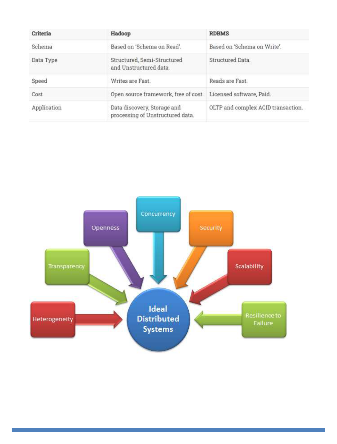
RDBMS Versus Hadoop
Distributed Computing Challenges
Designing a distributed system does not come as easy and straight forward. A number
of challenges need to be overcome in order to get the ideal system. The major challenges in
distributed systems are listed below:
1. Heterogeneity:
The Internet enables users to access services and run applications over a heterogeneous collection
of computers and networks. Heterogeneity (that is, variety and difference) applies to all of the
following:

BIG DATA ANALYTICS
18
o Hardware devices: computers, tablets, mobile phones, embedded devices, etc.
o Operating System: Ms Windows, Linux, Mac, Unix, etc.
o Network: Local network, the Internet, wireless network, satellite links, etc.
o Programming languages: Java, C/C++, Python, PHP, etc.
o Different roles of software developers, designers, system managers
Different programming languages use different representations for characters and data structures
such as arrays and records. These differences must be addressed if programs written in different
languages are to be able to communicate with one another. Programs written by different
developers cannot communicate with one another unless they use common standards, for example,
for network communication and the
representation of primitive data items and data structures in messages. For this to happen, standards
need to be agreed and adopted – as have the Internet protocols.
Middleware: The term middleware applies to a software layer that provides a programming
abstraction as well as masking the heterogeneity of the underlying networks, hardware, operating
systems and programming languages. Most middleware is implemented over the Internet
protocols, which themselves mask the differences of the underlying networks, but all middleware
deals with the differences in operating systems
and hardware
Heterogeneity and mobile code: The term mobile code is used to refer to program code that can
be transferred from one computer to another and run at the destination – Java applets are an
example. Code suitable for running on one computer is not necessarily suitable for running on
another because executable programs are normally specific both to the instruction set and to the
host operating system.
2. Transparency:
Transparency is defined as the concealment from the user and the application programmer of the
separation of components in a distributed system, so that the system is perceived as a whole rather
than as a collection of independent components. In other words, distributed systems designers must
hide the complexity of the systems as much as they can. Some terms of transparency in distributed
systems are:
Access Hide differences in data representation and how a resource is accessed
Location Hide where a resource is located
Migration Hide that a resource may move to another location
Relocation Hide that a resource may be moved to another location while in use
Replication Hide that a resource may be copied in several places
Concurrency Hide that a resource may be shared by several competitive users
Failure Hide the failure and recovery of a resource
Persistence Hide whether a (software) resource is in memory or a disk
3. Openness
The openness of a computer system is the characteristic that determines whether the system can
be extended and re-implemented in various ways. The openness of distributed systems is
determined primarily by the degree to which new resource-sharing services can be added and be

BIG DATA ANALYTICS
19
made available for use by a variety of client programs. If the well-defined interfaces for a system
are published, it is easier for developers to add new features or replace sub-systems in the future.
Example: Twitter and Facebook have API that allows developers to develop their own software
interactively.
4. Concurrency
Both services and applications provide resources that can be shared by clients in a distributed
system. There is therefore a possibility that several clients will attempt to access a shared resource
at the same time. For example, a data structure that records bids for an auction may be accessed
very frequently when it gets close to the deadline time. For an object to be safe in a concurrent
environment, its operations must be synchronized in such a way that its data remains consistent.
This can be achieved by standard techniques such as semaphores, which are used in most operating
systems.
5. Security
Many of the information resources that are made available and maintained in distributed systems
have a high intrinsic value to their users. Their security is therefore of considerable importance.
Security for information resources has three components:
confidentiality (protection against disclosure to unauthorized individuals)
integrity (protection against alteration or corruption),
availability for the authorized (protection against interference with the means to access the
resources).
6. Scalability
Distributed systems must be scalable as the number of user increases. The scalability is defined by
B. Clifford Neuman as
A system is said to be scalable if it can handle the addition of users and resources without suffering
a noticeable loss of performance or increase in administrative complexity
Scalability has 3 dimensions:
o Size
o Number of users and resources to be processed. Problem associated is overloading
o Geography
o Distance between users and resources. Problem associated is communication reliability
o Administration
o As the size of distributed systems increases, many of the system needs to be controlled.
Problem associated is administrative mess
7. Failure Handling
Computer systems sometimes fail. When faults occur in hardware or software, programs may
produce incorrect results or may stop before they have completed the intended computation. The
handling of failures is particularly difficult.
BIG DATA ANALYTICS
20
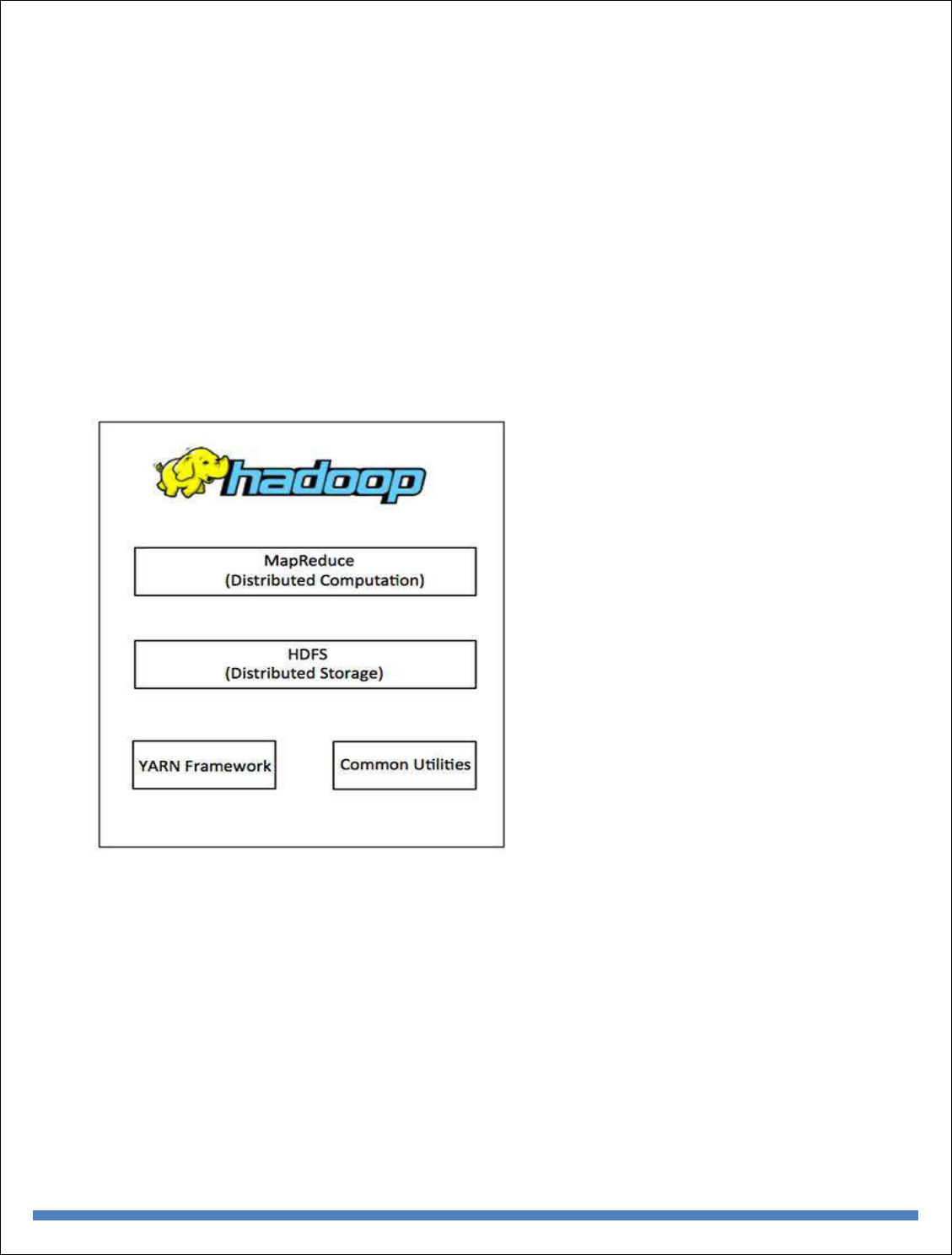
Hadoop Overview
Hadoop is an Apache open source framework written in java that allows distributed processing
of large datasets across clusters of computers using simple programming models. The Hadoop
framework application works in an environment that provides
distributed storage and computation across clusters of computers. Hadoop is designed to scale up
from single server to thousands of machines, each offering local computation and storage.
Hadoop Architecture
At its core, Hadoop has two major layers namely −
Processing/Computation layer (MapReduce), and
Storage layer (Hadoop Distributed File System).
MapReduce
MapReduce is a parallel programming model for writing distributed applications devised at
Google for efficient processing of large amounts of data (multi-terabyte data-sets), on large
clusters (thousands of nodes) of commodity hardware in a reliable, fault-tolerant manner. The
MapReduce program runs on Hadoop which is an Apache open-source framework.
Hadoop Distributed File System
The Hadoop Distributed File System (HDFS) is based on the Google File System (GFS) and
provides a distributed file system that is designed to run on commodity hardware. It has many

BIG DATA ANALYTICS
21
similarities with existing distributed file systems. However, the differences from other distributed
file systems are significant. It is highly fault-tolerant and is designed to be deployed on low-cost
hardware. It provides high throughput access to application data and is suitable for applications
having large datasets.
Apart from the above-mentioned two core components, Hadoop framework also includes the
following two modules −
Hadoop Common − These are Java libraries and utilities required by other Hadoop
modules.
Hadoop YARN − This is a framework for job scheduling and cluster resource
management.
How Does Hadoop Work?
It is quite expensive to build bigger servers with heavy configurations that handle large scale
processing, but as an alternative, you can tie together many commodity computers with single-
CPU, as a single functional distributed system and practically, the clustered machines can read
the dataset in parallel and provide a much higher throughput. Moreover, it is cheaper than one
high-end server. So this is the first motivational factor behind using Hadoop that it runs across
clustered and low-cost machines.
Hadoop runs code across a cluster of computers. This process includes the following core tasks
that Hadoop performs −
Data is initially divided into directories and files. Files are divided into uniform sized
blocks of 128M and 64M (preferably 128M).
These files are then distributed across various cluster nodes for further processing.
HDFS, being on top of the local file system, supervises the processing.
Blocks are replicated for handling hardware failure.
Checking that the code was executed successfully.
Performing the sort that takes place between the map and reduce stages.
Sending the sorted data to a certain computer.
Writing the debugging logs for each job.
Advantages of Hadoop
Hadoop framework allows the user to quickly write and test distributed systems. It is
efficient, and it automatic distributes the data and work across the machines and in turn,
utilizes the underlying parallelism of the CPU cores.

BIG DATA ANALYTICS
22
Hadoop does not rely on hardware to provide fault-tolerance and high availability (FTHA),
rather Hadoop library itself has been designed to detect and handle failures at the
application layer.
Servers can be added or removed from the cluster dynamically and Hadoop continues to
operate without interruption.
Another big advantage of Hadoop is that apart from being open source, it is compatible on
all the platforms since it is Java based.
Processing Data with Hadoop - Managing Resources and Applications with Hadoop YARN
Yarn divides the task on resource management and job scheduling/monitoring into separate
daemons. There is one ResourceManager and per-application ApplicationMaster. An application
can be either a job or a DAG of jobs.
The ResourceManger have two components – Scheduler and AppicationManager.
The scheduler is a pure scheduler i.e. it does not track the status of running application. It only
allocates resources to various competing applications. Also, it does not restart the job after failure
due to hardware or application failure. The scheduler allocates the resources based on an abstract
notion of a container. A container is nothing but a fraction of resources like CPU, memory, disk,
network etc.
Following are the tasks of ApplicationManager:-
Accepts submission of jobs by client.
Negotaites first container for specific ApplicationMaster.
Restarts the container after application failure.
Below are the responsibilities of ApplicationMaster
Negotiates containers from Scheduler
Tracking container status and monitoring its progress.
Yarn supports the concept of Resource Reservation via Reservation System. In this, a user can fix
a number of resources for execution of a particular job over time and temporal constraints. The
Reservation System makes sure that the resources are available to the job until its completion. It
also performs admission control for reservation.
Yarn can scale beyond a few thousand nodes via Yarn Federation. YARN Federation allows to
wire multiple sub-cluster into the single massive cluster. We can use many independent clusters
together for a single large job. It can be used to achieve a large scale system.
Let us summarize how Hadoop works step by step:
Input data is broken into blocks of size 128 Mb and then blocks are moved to different nodes.
Once all the blocks of the data are stored on data-nodes, the user can process the data.
Resource Manager then schedules the program (submitted by the user) on individual nodes.
Once all the nodes process the data, the output is written back to HDFS.

BIG DATA ANALYTICS
23
Interacting with Hadoop Ecosystem
Hadoop Ecosystem Hadoop has an ecosystem that has evolved from its three core components
processing, resource management, and storage. In this topic, you will learn the components of the
Hadoop ecosystem and how they perform their roles during Big Data processing. The
Hadoop ecosystem is continuously growing to meet the needs of Big Data. It comprises the
following twelve components:
HDFS(Hadoop Distributed file system)
HBase
Sqoop
Flume
Spark
Hadoop MapReduce
Pig
Impala
Hive
Cloudera Search
Oozie
Hue.
Let us understand the role of each component of the Hadoop ecosystem.
Components of Hadoop Ecosystem
Let us start with the first component HDFS of Hadoop Ecosystem.
HDFS (HADOOP DISTRIBUTED FILE SYSTEM)
HDFS is a storage layer for Hadoop.
HDFS is suitable for distributed storage and processing, that is, while the data is being
stored, it first gets distributed and then it is processed.
HDFS provides Streaming access to file system data.
HDFS provides file permission and authentication.
HDFS uses a command line interface to interact with Hadoop.
So what stores data in HDFS? It is the HBase which stores data in HDFS.
HBase
HBase is a NoSQL database or non-relational database .
HBase is important and mainly used when you need random, real-time, read, or write
access to your Big Data.
It provides support to a high volume of data and high throughput.
In an HBase, a table can have thousands of columns.

BIG DATA ANALYTICS
24
UNIT-III
INTRODUCTION TO MONGODB AND MAPREDUCE PROGRAMMING
MongoDB is a cross-platform, document-oriented database that provides, high performance, high
availability, and easy scalability. MongoDB works on concept of collection and document.
Database
Database is a physical container for collections. Each database gets its own set of files on the file
system. A single MongoDB server typically has multiple databases.
Collection
Collection is a group of MongoDB documents. It is the equivalent of an RDBMS table. A
collection exists within a single database. Collections do not enforce a schema. Documents within
a collection can have different fields. Typically, all documents in a collection are of similar or
related purpose.
Document
A document is a set of key-value pairs. Documents have dynamic schema. Dynamic schema means
that documents in the same collection do not need to have the same set of fields or structure, and
common fields in a collection's documents may hold different types of data.
The following table shows the relationship of RDBMS terminology with MongoDB.
RDBMS
MongoDB
Database
Database
Table
Collection
Tuple/Row
Document
column
Field
Table Join
Embedded Documents

BIG DATA ANALYTICS
25
Primary Key
Primary Key (Default key _id provided by
MongoDB itself)
Database Server and Client
mysqld/Oracle
mongod
mysql/sqlplus
mongo
Sample Document
Following example shows the document structure of a blog site, which is simply a comma
separated key value pair.
{
_id: ObjectId(7df78ad8902c)
title: 'MongoDB Overview',
description: 'MongoDB is no sql database',
by: 'tutorials point',
url: 'http://www.tutorialspoint.com',
tags: ['mongodb', 'database', 'NoSQL'],
likes: 100,
comments: [
{
user:'user1',
message: 'My first comment',
dateCreated: new Date(2011,1,20,2,15),
like: 0

BIG DATA ANALYTICS
26
},
{
user:'user2',
message: 'My second comments',
dateCreated: new Date(2011,1,25,7,45),
like: 5
}
]
}
_id is a 12 bytes hexadecimal number which assures the uniqueness of every document. You can
provide _id while inserting the document. If you don’t provide then MongoDB provides a unique
id for every document. These 12 bytes first 4 bytes for the current timestamp, next 3 bytes for
machine id, next 2 bytes for process id of MongoDB server and remaining 3 bytes are simple
incremental VALUE.
Any relational database has a typical schema design that shows number of tables and the
relationship between these tables. While in MongoDB, there is no concept of relationship.
Advantages of MongoDB over RDBMS
Schema less − MongoDB is a document database in which one collection holds different
documents. Number of fields, content and size of the document can differ from one
document to another.
Structure of a single object is clear.
No complex joins.
Deep query-ability. MongoDB supports dynamic queries on documents using a document-
based query language that's nearly as powerful as SQL.
Tuning.
Ease of scale-out − MongoDB is easy to scale.
Conversion/mapping of application objects to database objects not needed.
Uses internal memory for storing the (windowed) working set, enabling faster access of
data.

BIG DATA ANALYTICS
27
Why Use MongoDB?
Document Oriented Storage − Data is stored in the form of JSON style documents.
Index on any attribute
Replication and high availability
Auto-Sharding
Rich queries
Fast in-place updates
Professional support by MongoDB
Where to Use MongoDB?
Big Data
Content Management and Delivery
Mobile and Social Infrastructure
User Data Management
Data Hub
MongoDB supports many datatypes. Some of them are −
String − This is the most commonly used datatype to store the data. String in MongoDB
must be UTF-8 valid.
Integer − This type is used to store a numerical value. Integer can be 32 bit or 64 bit
depending upon your server.
Boolean − This type is used to store a boolean (true/ false) value.
Double − This type is used to store floating point values.
Min/ Max keys − This type is used to compare a value against the lowest and highest
BSON elements.
Arrays − This type is used to store arrays or list or multiple values into one key.
Timestamp − ctimestamp. This can be handy for recording when a document has been
modified or added.
Object − This datatype is used for embedded documents.
Null − This type is used to store a Null value.
Symbol − This datatype is used identically to a string; however, it's generally reserved for
languages that use a specific symbol type.
Date − This datatype is used to store the current date or time in UNIX time format. You
can specify your own date time by creating object of Date and passing day, month, year
into it.
Object ID − This datatype is used to store the document’s ID.

BIG DATA ANALYTICS
28
Binary data − This datatype is used to store binary data.
Code − This datatype is used to store JavaScript code into the document.
Regular expression − This datatype is used to store regular expression.
The find() Method
To query data from MongoDB collection, you need to use MongoDB's find() method.
Syntax
The basic syntax of find() method is as follows −
>db.COLLECTION_NAME.find()
find() method will display all the documents in a non-structured way.
Example
Assume we have created a collection named mycol as −
> use sampleDB
switched to db sampleDB
> db.createCollection("mycol")
{ "ok" : 1 }
>
And inserted 3 documents in it using the insert() method as shown below −
> db.mycol.insert([
{
title: "MongoDB Overview",
description: "MongoDB is no SQL database",
by: "tutorials point",
url: "http://www.tutorialspoint.com",
tags: ["mongodb", "database", "NoSQL"],
likes: 100
},
{
title: "NoSQL Database",
description: "NoSQL database doesn't have tables",
by: "tutorials point",
url: "http://www.tutorialspoint.com",
tags: ["mongodb", "database", "NoSQL"],
likes: 20,
comments: [

BIG DATA ANALYTICS
29
{
user:"user1",
message: "My first comment",
dateCreated: new Date(2013,11,10,2,35),
like: 0
}
]
}
])
Following method retrieves all the documents in the collection −
> db.mycol.find()
{ "_id" : ObjectId("5dd4e2cc0821d3b44607534c"), "title" : "MongoDB Overview", "description"
: "MongoDB is no SQL database", "by" : "tutorials point", "url" : "http://www.tutorialspoint.com",
"tags" : [ "mongodb", "database", "NoSQL" ], "likes" : 100 }
{ "_id" : ObjectId("5dd4e2cc0821d3b44607534d"), "title" : "NoSQL Database", "description" :
"NoSQL database doesn't have tables", "by" : "tutorials point", "url" :
"http://www.tutorialspoint.com", "tags" : [ "mongodb", "database", "NoSQL" ], "likes" : 20,
"comments" : [ { "user" : "user1", "message" : "My first comment", "dateCreated" :
ISODate("2013-12-09T21:05:00Z"), "like" : 0 } ] }
>
The pretty() Method
To display the results in a formatted way, you can use pretty() method.
Syntax
>db.COLLECTION_NAME.find().pretty()
Example
Following example retrieves all the documents from the collection named mycol and arranges
them in an easy-to-read format.
> db.mycol.find().pretty()
{
"_id" : ObjectId("5dd4e2cc0821d3b44607534c"),
"title" : "MongoDB Overview",
"description" : "MongoDB is no SQL database",
"by" : "tutorials point",
"url" : "http://www.tutorialspoint.com",
"tags" : [
"mongodb",
"database",
"NoSQL"
],
"likes" : 100

BIG DATA ANALYTICS
30
}
{
"_id" : ObjectId("5dd4e2cc0821d3b44607534d"),
"title" : "NoSQL Database",
"description" : "NoSQL database doesn't have tables",
"by" : "tutorials point",
"url" : "http://www.tutorialspoint.com",
"tags" : [
"mongodb",
"database",
"NoSQL"
],
"likes" : 20,
"comments" : [
{
"user" : "user1",
"message" : "My first comment",
"dateCreated" : ISODate("2013-12-09T21:05:00Z"),
"like" : 0
}
]
}
The findOne() method
Apart from the find() method, there is findOne() method, that returns only one document.
Syntax
>db.COLLECTIONNAME.findOne()
Example
Following example retrieves the document with title MongoDB Overview.
> db.mycol.findOne({title: "MongoDB Overview"})
{
"_id" : ObjectId("5dd6542170fb13eec3963bf0"),
"title" : "MongoDB Overview",
"description" : "MongoDB is no SQL database",
"by" : "tutorials point",
"url" : "http://www.tutorialspoint.com",
"tags" : [
"mongodb",
"database",
"NoSQL"
],
"likes" : 100
BIG DATA ANALYTICS
31
}
RDBMS Where Clause Equivalents in MongoDB
To query the document on the basis of some condition, you can use following operations.
Operation
Syntax
Example
RDBMS
Equivalent
Equality
{<key>:{$eg;<value>}}
db.mycol.find({"by":"tutorials
point"}).pretty()
where by =
'tutorials
point'
Less Than
{<key>:{$lt:<value>}}
db.mycol.find({"likes":{$lt:50}}).pretty()
where likes
< 50
Less Than
Equals
{<key>:{$lte:<value>}}
db.mycol.find({"likes":{$lte:50}}).pretty()
where likes
<= 50
Greater
Than
{<key>:{$gt:<value>}}
db.mycol.find({"likes":{$gt:50}}).pretty()
where likes
> 50
Greater
Than
Equals
{<key>:{$gte:<value>}}
db.mycol.find({"likes":{$gte:50}}).pretty()
where likes
>= 50
Not
Equals
{<key>:{$ne:<value>}}
db.mycol.find({"likes":{$ne:50}}).pretty()
where likes
!= 50
Values in
an array
{<key>:{$in:[<value1>,
<value2>,……<valueN>]}}
db.mycol.find({"name":{$in:["Raj",
"Ram", "Raghu"]}}).pretty()
Where
name
matches
any of the
value in
:["Raj",
"Ram",
"Raghu"]

BIG DATA ANALYTICS
32
Values not
in an array
{<key>:{$nin:<value>}}
db.mycol.find({"name":{$nin:["Ramu",
"Raghav"]}}).pretty()
Where
name
values is
not in the
array
:["Ramu",
"Raghav"]
or, doesn’t
exist at all
AND in MongoDB
Syntax
To query documents based on the AND condition, you need to use $and keyword. Following is
the basic syntax of AND −
>db.mycol.find({ $and: [ {<key1>:<value1>}, { <key2>:<value2>} ] })
Example
Following example will show all the tutorials written by 'tutorials point' and whose title is
'MongoDB Overview'.
> db.mycol.find({$and:[{"by":"tutorials point"},{"title": "MongoDB Overview"}]}).pretty()
{
"_id" : ObjectId("5dd4e2cc0821d3b44607534c"),
"title" : "MongoDB Overview",
"description" : "MongoDB is no SQL database",
"by" : "tutorials point",
"url" : "http://www.tutorialspoint.com",
"tags" : [
"mongodb",
"database",
"NoSQL"
],
"likes" : 100
}
>
For the above given example, equivalent where clause will be ' where by = 'tutorials point'
AND title = 'MongoDB Overview' '. You can pass any number of key, value pairs in find clause.
OR in MongoDB
Syntax

BIG DATA ANALYTICS
33
To query documents based on the OR condition, you need to use $or keyword. Following is the
basic syntax of OR −
>db.mycol.find(
{
$or: [
{key1: value1}, {key2:value2}
]
}
).pretty()
Example
Following example will show all the tutorials written by 'tutorials point' or whose title is
'MongoDB Overview'.
>db.mycol.find({$or:[{"by":"tutorials point"},{"title": "MongoDB Overview"}]}).pretty()
{
"_id": ObjectId(7df78ad8902c),
"title": "MongoDB Overview",
"description": "MongoDB is no sql database",
"by": "tutorials point",
"url": "http://www.tutorialspoint.com",
"tags": ["mongodb", "database", "NoSQL"],
"likes": "100"
}
>
Using AND and OR Together
Example
The following example will show the documents that have likes greater than 10 and whose title
is either 'MongoDB Overview' or by is 'tutorials point'. Equivalent SQL where clause is 'where
likes>10 AND (by = 'tutorials point' OR title = 'MongoDB Overview')'
>db.mycol.find({"likes": {$gt:10}, $or: [{"by": "tutorials point"},
{"title": "MongoDB Overview"}]}).pretty()
{
"_id": ObjectId(7df78ad8902c),
"title": "MongoDB Overview",
"description": "MongoDB is no sql database",
"by": "tutorials point",
"url": "http://www.tutorialspoint.com",
"tags": ["mongodb", "database", "NoSQL"],
"likes": "100"
}
>

BIG DATA ANALYTICS
34
NOR in MongoDB
Syntax
To query documents based on the NOT condition, you need to use $not keyword. Following is
the basic syntax of NOT −
>db.COLLECTION_NAME.find(
{
$not: [
{key1: value1}, {key2:value2}
]
}
)
Example
Assume we have inserted 3 documents in the collection empDetails as shown below −
db.empDetails.insertMany(
[
{
First_Name: "Radhika",
Last_Name: "Sharma",
Age: "26",
e_mail: "radhika_sharma.123@gmail.com",
phone: "9000012345"
},
{
First_Name: "Rachel",
Last_Name: "Christopher",
Age: "27",
e_mail: "Rachel_Christopher.123@gmail.com",
phone: "9000054321"
},
{
First_Name: "Fathima",
Last_Name: "Sheik",
Age: "24",
e_mail: "Fathima_Sheik.123@gmail.com",
phone: "9000054321"
}
]
)
Following example will retrieve the document(s) whose first name is not "Radhika" and last name
is not "Christopher"
> db.empDetails.find(
{

BIG DATA ANALYTICS
35
$nor:[
40
{"First_Name": "Radhika"},
{"Last_Name": "Christopher"}
]
}
).pretty()
{
"_id" : ObjectId("5dd631f270fb13eec3963bef"),
"First_Name" : "Fathima",
"Last_Name" : "Sheik",
"Age" : "24",
"e_mail" : "Fathima_Sheik.123@gmail.com",
"phone" : "9000054321"
}
NOT in MongoDB
Syntax
To query documents based on the NOT condition, you need to use $not keyword following is the
basic syntax of NOT −
>db.COLLECTION_NAME.find(
{
$NOT: [
{key1: value1}, {key2:value2}
]
}
).pretty()
Example
Following example will retrieve the document(s) whose age is not greater than 25
> db.empDetails.find( { "Age": { $not: { $gt: "25" } } } )
{
"_id" : ObjectId("5dd6636870fb13eec3963bf7"),
"First_Name" : "Fathima",
"Last_Name" : "Sheik",
"Age" : "24",
"e_mail" : "Fathima_Sheik.123@gmail.com",
"phone" : "9000054321"
}

BIG DATA ANALYTICS
36
MapReduce:
MapReduce addresses the challenges of distributed programming by providing an abstraction that
isolates the developer from system-level details (e.g., locking of data structures, data starvation
issues in the processing pipeline, etc.). The programming model specifies simple and well-defined
interfaces between a small number of components, and therefore is easy for the programmer to
reason about. MapReduce maintains a separation of what computations are to be performed and
how those computations are actually carried out on a cluster of machines. The first is under the
control of the programmer, while the second is exclusively the responsibility of the execution
framework or “runtime”. The advantage is that the execution framework only needs to be designed
once and verified for correctness—thereafter, as long as the developer expresses computations in
the programming model, code is guaranteed to behave as expected. The upshot is that the developer
is freed from having to worry about system-level details (e.g., no more debugging race conditions
and addressing lock contention) and can instead focus on algorithm or application design.
ich often has multiple cores). Why is MapReduce important? In practical terms, it provides a very
effective tool for tackling large-data problems. But beyond that, MapReduce is important in how
it has changed the way we organize computations at a massive scale. MapReduce represents the
first widely-adopted step away from the von Neumann model that has served as the foundation of
computer science over the last half plus century. Valiant called this a bridging model [148], a
conceptual bridge between the physical implementation of a machine and the software that is to
be executed on that machine. Until recently, the von Neumann model has served us well: Hardware
designers focused on efficient implementations of the von Neumann model and didn’t have to
think much about the actual software that would run on the machines. Similarly, the software
industry developed software targeted at the model without worrying about the hardware details.
The result was extraordinary growth: chip designers churned out successive generations of
increasingly powerful processors, and software engineers were able to develop applications in
high-level languages that exploited those processors.
MapReduce can be viewed as the first breakthrough in the quest for new abstractions that allow us
to organize computations, not over individual machines, but over entire clusters. As Barroso puts
it, the datacenter is the computer. MapReduce is certainly not the first model of parallel
computation that has been proposed. The most prevalent model in theoretical computer science,
which dates back several decades, is the PRAM. MAPPERS AND REDUCERS Key-value pairs
form the basic data structure in MapReduce. Keys and values may be primitives such as integers,
floating point values, strings, and raw bytes, or they may be arbitrarily complex structures (lists,
tuples, associative arrays, etc.). Programmers typically need to define their own custom data types,
although a number of libraries such as Protocol Buffers,5 Thrift,6 and Avro7 simplify the task.
Part of the design of MapReduce algorithms involves imposing the key-value structure on arbitrary
datasets. For a collection of web pages, keys may be URLs and values may be the actual HTML
content. For a graph, keys may represent node ids and values may contain the adjacency lists of
those nodes (see Chapter 5 for more details). In some algorithms, input keys are not particularly
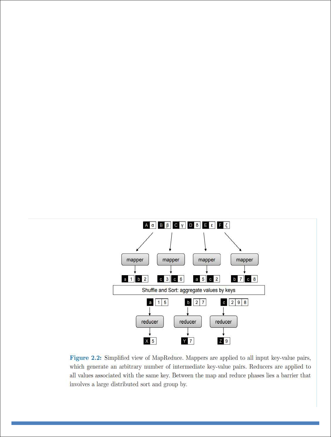
BIG DATA ANALYTICS
37
meaningful and are simply ignored during processing, while in other cases input keys are used to
uniquely identify a datum (such as a record id). In Chapter 3, we discuss the role of complex keys
and values in the design of various algorithms. In MapReduce, the programmer defines a mapper
and a reducer with the following signatures: map: (k1, v1) → [(k2, v2)] reduce: (k2, [v2]) → [(k3,
v3)] The convention [. . .] is used throughout this book to denote a list. The input to a MapReduce
job starts as data stored on the underlying distributed file system (see Section 2.5). The mapper is
applied to every input key-value pair (split across an arbitrary number of files) to generate an
arbitrary number of intermediate key-value pairs. The reducer is applied to all values associated
with the same intermediate key to generate output key-value pairs.8 Implicit between the map and
reduce phases is a distributed “group by” operation on intermediate keys. Intermediate data arrive
at each reducer in order, sorted by the key. However, no ordering relationship is guaranteed for
keys across different reducers. Output key-value pairs from each reducer are written persistently
back onto the distributed file system (whereas intermediate key-value pairs are transient and not
preserved). The output ends up in r files on the distributed file system, where r is the number of
reducers. For the most part, there is no need to consolidate reducer output, since the r files often
serve as input to yet another MapReduce job. Figure 2.2 illustrates this two-stage processing
structure. A simple word count algorithm in MapReduce is shown in Figure 2.3. This algorithm
counts the number of occurrences of every word in a text collection, which may be the first step
in, for example, building a unigram language model (i.e., probability

BIG DATA ANALYTICS
38
MAPREDUCE BASICS
distribution over words in a collection). Input key-values pairs take the form of (docid, doc) pairs
stored on the distributed file system, where the former is a unique identifier for the document, and
the latter is the text of the document itself. The mapper takes an input key-value pair, tokenizes
the document, and emits an intermediate key-value pair for every word: the word itself serves as
the key, and the integer one serves as the value (denoting that we’ve seen the word once). The
MapReduce execution framework guarantees that all values associated with the same key are
brought together in the reducer. Therefore, in our word count algorithm, we simply need to sum
up all counts (ones) associated with each word. The reducer does exactly this, and emits final
keyvalue pairs with the word as the key, and the count as the value. Final output is written to the
distributed file system, one file per reducer. Words within each file will be sorted by alphabetical
order, and each file will contain roughly the same number of words. The partitioner, which we
discuss later in Section 2.4, controls the assignment of words to reducers. The output can be
examined by the programmer or used as input to another MapReduce program.
There are some differences between the Hadoop implementation of MapReduce and Google’s
implementation.9 In Hadoop, the reducer is presented with a key and an iterator over all values
associated with the particular key. The values are arbitrarily ordered. Google’s implementation
allows the programmer to specify a secondary sort key for ordering the values (if desired)—in
which case values associated with each key would be presented to the developer’s reduce code in
sorted order. Later in Section 3.4 we discuss how to overcome this limitation in Hadoop to perform
secondary sorting. Another difference: in Google’s implementation the programmer is not allowed
to change the key in the reducer. That is, the reducer output key must be exactly the same as the
reducer input key. In Hadoop, there is no such restriction, and the reducer can emit an arbitrary
number of output key-value pairs (with different keys).
To provide a bit more implementation detail: pseudo-code provided in this book roughly mirrors
how MapReduce programs are written in Hadoop. Mappers and reducers are objects that
implement the Map and Reduce methods, respectively. In Hadoop, a mapper object is initialized
for each map task (associated with a particular sequence of key-value pairs called an input split)
and the Map method is called on each key-value pair by the execution framework. In configuring
a MapReduce job, the programmer provides a hint on the number of map tasks to run, but the
execution framework (see next section) makes the final determination based on the physical layout
of the data (more details in Section 2.5 and Section 2.6). The situation is similar for the reduce
phase: a reducer object is initialized for each reduce task, and the Reduce method is called once
per intermediate key. In contrast with the number of map tasks, the programmer can precisely
specify the number of reduce tasks. We will return to discuss the details of Hadoop job execution
in Section 2.6, which is dependent on an understanding of the distributed file system (covered in
Section 2.5). To reiterate: although the presentation of algorithms in this book closely mirrors the
way they would be implemented in Hadoop, our focus is on algorithm design and conceptual

BIG DATA ANALYTICS
39
understanding—not actual Hadoop programming. For that, we would recommend Tom White’s
book [154]. What are the restrictions on mappers and reducers? Mappers and reducers can express
arbitrary computations over their inputs. However, one must generally be careful about use of
external resources since multiple mappers or reducers may be contending for those resources. For
example, it may be unwise for a mapper to query an external SQL database, since that would
introduce a scalability bottleneck on the number of map tasks that could be run in parallel (since
they might all be simultaneously querying the database).10 In general, mappers can emit an
arbitrary number of intermediate key-value pairs, and they need not be of the same type as the
input key-value pairs. Similarly, reducers can emit an arbitrary number of final key-value pairs,
and they can differ in type from the intermediate key-value pairs. Although not permitted in
functional programming, mappers and reducers can have side effects. This is a powerful and useful
feature: for example, preserving state across multiple inputs is central to the design of many
MapReduce algorithms (see Chapter 3). Such algorithms can be understood as having side effects
that only change state that is internal to the mapper or reducer. While the correctness of such
algorithms may be more difficult to guarantee (since the function’s behavior depends not only on
the current input but on previous inputs), most potential synchronization problems are avoided
since internal state is private only to individual mappers and reducers. In other cases (see Section
4.4 and Section 6.5), it may be useful for mappers or reducers to have external side effects, such
as writing files to the distributed file system. Since many mappers and reducers are run in parallel,
and the distributed file system is a shared global resource, special care must be taken to ensure that
such operations avoid synchronization conflicts. One strategy is to write a temporary file that is
renamed upon successful completion of the mapper or reducer .
In addition to the “canonical” MapReduce processing flow, other variations are also possible.
MapReduce programs can contain no reducers, in which case mapper output is directly written to
disk (one file per mapper). For embarrassingly parallel problems, e.g., parse a large text collection
or independently analyze a large number of images, this would be a common pattern. The
converse—a MapReduce program with no mappers—is not possible, although in some cases it is
useful for the mapper to implement the identity function and simply pass input key-value pairs to
the reducers. This has the effect of sorting and regrouping the input for reduce-side processing.
Similarly, in some cases it is useful for the reducer to implement the identity function, in which
case the program simply sorts and groups mapper output. Finally, running identity mappers and
reducers has the effect of regrouping and resorting the input data (which is sometimes useful).
Although in the most common case, input to a MapReduce job comes from data stored on the
distributed file system and output is written back to the distributed file system, any other system
that satisfies the proper abstractions can serve as a data source or sink. With Google’s MapReduce
implementation, BigTable [34], a sparse, distributed, persistent multidimensional sorted map, is
frequently used as a source of input and as a store of MapReduce output. HBase is an open-source
BigTable clone and has similar capabilities. Also, Hadoop has been integrated with existing MPP
(massively parallel processing) relational databases, which allows a programmer to write
MapReduce jobs over database rows and dump output into a new database table. Finally, in some

BIG DATA ANALYTICS
40
cases MapReduce jobs may not consume any input at all (e.g., computing π) or may only consume
a small amount of data (e.g., input parameters to many instances of processorintensive simulations
running in parallel).
PARTITIONERS AND COMBINERS
We have thus far presented a simplified view of MapReduce. There are two additional elements
that complete the programming model: partitioners and combiners. Partitioners are responsible for
dividing up the intermediate key space and assigning intermediate key-value pairs to reducers. In
other words, the partitioner specifies the task to which an intermediate key-value pair must be
copied. Within each reducer, keys are processed in sorted order (which is how the “group by” is
implemented). The simplest partitioner involves computing the hash value of the key and then
taking the mod of that value with the number of reducers. This assigns approximately the same
number of keys to each reducer (dependent on the quality of the hash function). Note, however,
that the partitioner only considers the key and ignores the value—therefore, a roughly-even
partitioning of the key space may nevertheless yield large differences in the number of key-values
pairs sent to each reducer (since different keys may have different numbers of associated values).
This imbalance in the amount of data associated with each key is relatively common in many text
processing applications due to the Zipfian distribution of word occurrences.
Combiners are an optimization in MapReduce that allow for local aggregation before the shuffle
and sort phase. We can motivate the need for combiners by considering the word count algorithm
in Figure 2.3, which emits a key-value pair for each word in the collection. Furthermore, all these
key-value pairs need to be copied across the network, and so the amount of intermediate data will
be larger than the input collection itself. This is clearly inefficient. One solution is to perform local
aggregation on the output of each mapper, i.e., to compute a local count for a word over all the
documents processed by the mapper. With this modification (assuming the maximum amount of
local aggregation possible), the number of intermediate key-value pairs will be at most the number
of unique words in the collection times the number of mappers (and typically far smaller because
each mapper may not encounter every word).
smaller because each mapper may not encounter every word). The combiner in MapReduce
supports such an optimization. One can think of combiners as “mini-reducers” that take place on
the output of the mappers, prior to the shuffle and sort phase. Each combiner operates in isolation
and therefore does not have access to intermediate output from other mappers. The combiner is
provided keys and values associated with each key (the same types as the mapper output keys and
values). Critically, one cannot assume that a combiner will have the opportunity to process all
values associated with the same key. The combiner can emit any number of key-value pairs, but
the keys and values must be of the same type as the mapper output (same as the reducer input).12
In cases where an operation is both associative and commutative (e.g., addition or multiplication),
reducers can directly serve as combiners. In general, however, reducers and combiners are not
interchangeable.
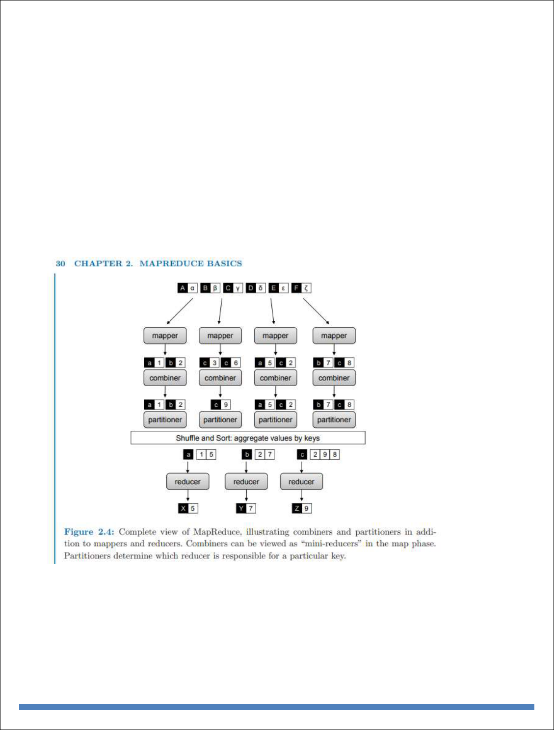
BIG DATA ANALYTICS
41
In many cases, proper use of combiners can spell the difference between an impractical algorithm
and an efficient algorithm. This topic will be discussed in Section 3.1, which focuses on various
techniques for local aggregation. It suffices to say for now that a combiner can significantly reduce
the amount of data that needs to be copied over the network, resulting in much faster algorithms.
The complete MapReduce model is shown in Figure 2.4. Output of the mappers are processed by
the combiners, which perform local aggregation to cut down on the number of intermediate key-
value pairs. The partitioner determines which reducer will be responsible for processing a
particular key, and the execution framework uses this information to copy the data to the right
location during the shuffle and sort phase.13 Therefore, a complete MapReduce job consists of
code for the mapper, reducer, combiner, and partitioner, along with job configuration parameters.
The execution framework handles everything else.
SECONDARY SORTING
MapReduce sorts intermediate key-value pairs by the keys during the shuffle and sort phase, which
is very convenient if computations inside the reducer rely on sort order (e.g., the order inversion
design pattern described in the previous section). However, what if in addition to sorting by key,
we also need to sort by value? Google’s MapReduce implementation provides built-in

BIG DATA ANALYTICS
42
functionality for (optional) secondary sorting, which guarantees that values arrive in sorted order.
Hadoop, unfortunately, does not have this capability built in.
Consider the example of sensor data from a scientific experiment: there are m sensors each taking
readings on continuous basis, where m is potentially a large number. A dump of the sensor data
might look something like the following, where rx after each timestamp represents the actual
sensor readings (unimportant for this discussion, but may be a series of values, one or more
complex records, or even raw bytes of images).
(t1, m1, r80521)
(t1, m2, r14209)
(t1, m3, r76042) ...
(t2, m1, r21823)
(t2, m2, r66508)
(t2, m3, r98347)
Suppose we wish to reconstruct the activity at each individual sensor over time. A MapReduce
program to accomplish this might map over the raw data and emit the sensor id as the intermediate
key, with the rest of each record as the value:
m1 → (t1, r80521)
This would bring all readings from the same sensor together in the reducer. However, since
MapReduce makes no guarantees about the ordering of values associated with the same key, the
sensor readings will not likely be in temporal order. The most obvious solution is to buffer all the
readings in memory and then sort by timestamp before additional processing. However, it should
be apparent by now that any in-memory buffering of data introduces a potential scalability
bottleneck. What if we are working with a high frequency sensor or sensor readings over a long
period of time? What if the sensor readings themselves are large complex objects? This approach
may not scale in these cases—the reducer would run out of memory trying to buffer all values
associated with the same key.
This is a common problem, since in many applications we wish to first group together data one
way (e.g., by sensor id), and then sort within the groupings another way (e.g., by time). Fortunately,
there is a general purpose solution, which we call the “value-to-key conversion” design pattern.
The basic idea is to move part of the value into the intermediate key to form a composite key, and
let the MapReduce execution framework handle the sorting. In the above example, instead of
emitting the sensor id as the key, we would emit the sensor id and the timestamp as a composite
key: (m1, t1) → (r80521)

BIG DATA ANALYTICS
43
The sensor reading itself now occupies the value. We must define the intermediate key sort order
to first sort by the sensor id (the left element in the pair) and then by the timestamp (the right
element in the pair). We must also implement a custom partitioner so that all pairs associated with
the same sensor are shuffled to the same reducer. Properly orchestrated, the key-value pairs will
be presented to the reducer in the correct sorted order: (m1, t1) → [(r80521)] (m1, t2) → [(r21823)]
(m1, t3) → [(r146925)] . . .
However, note that sensor readings are now split across multiple keys. The reducer will need to
preserve state and keep track of when readings associated with the current sensor end and the next
sensor begin.9 The basic tradeoff between the two approaches discussed above (buffer and
inmemory sort vs. value-to-key conversion) is where sorting is performed. One can explicitly
implement secondary sorting in the reducer, which is likely to be faster but suffers from a
scalability bottleneck.10 With value-to-key conversion, sorting is offloaded to the MapReduce
execution framework. Note that this approach can be arbitrarily extended to tertiary, quaternary,
etc. sorting. This pattern results in many more keys for the framework to sort, but distributed
sorting is a task that the MapReduce runtime excels at since it lies at the heart of the programming
model.
INDEX COMPRESSION
We return to the question of how postings are actually compressed and stored on disk. This chapter
devotes a substantial amount of space to this topic because index compression is one of the main
differences between a “toy” indexer and one that works on real-world collections. Otherwise,
MapReduce inverted indexing algorithms are pretty straightforward.
Let us consider the canonical case where each posting consists of a document id and the term
frequency. A na¨ıve implementation might represent the first as a 32-bit integer9 and the second
as a 16-bit integer. Thus, a postings list might be encoded as follows: [(5, 2),(7, 3),(12, 1),(49,
1),(51, 2), . . .]
where each posting is represented by a pair in parentheses. Note that all brackets, parentheses, and
commas are only included to enhance readability; in reality the postings would be represented as
a long stream of integers. This na¨ıve implementation would require six bytes per posting. Using
this scheme, the entire inverted index would be about as large as the collection itself. Fortunately,
we can do significantly better. The first trick is to encode differences between document ids as
opposed to the document ids themselves. Since the postings are sorted by document ids, the
differences (called d-gaps) must be positive integers greater than zero. The above postings list,
represented with d-gaps, would be: [(5, 2),(2, 3),(5, 1),(37, 1),(2, 2)
Of course, we must actually encode the first document id. We haven’t lost any information, since
the original document ids can be easily reconstructed from the d-gaps. However, it’s not obvious
that we’ve reduced the space requirements either, since the largest possible d-gap is one less than

BIG DATA ANALYTICS
44
the number of documents in the collection. This is where the second trick comes in, which is to
represent the d-gaps in a way such that it takes less space for smaller numbers. Similarly, we want
to apply the same techniques to compress the term frequencies, since for the most part they are
also small values. But to understand how this is done, we need to take a slight detour into
compression techniques, particularly for coding integers.
Compression, in general, can be characterized as either lossless or lossy: it’s fairly obvious that
loseless compression is required in this context. To start, it is important to understand that all
compression techniques represent a time–space tradeoff. That is, we reduce the amount of space
on disk necessary to store data, but at the cost of extra processor cycles that must be spent coding
and decoding data. Therefore, it is possible that compression reduces size but also slows
processing. However, if the two factors are properly balanced (i.e., decoding speed can keep up
with disk bandwidth), we can achieve the best of both worlds: smaller and faster.
POSTINGS COMPRESSION
Having completed our slight detour into integer compression techniques, we can now return to the
scalable inverted indexing algorithm shown in Figure 4.4 and discuss how postings lists can be
properly compressed. As we can see from the previous section, there is a wide range of choices
that represent different tradeoffs between compression ratio and decoding speed. Actual
performance also depends on characteristics of the collection, which, among other factors,
determine the distribution of d-gaps. B¨uttcher et al. [30] recently compared the performance of
various compression techniques on coding document ids. In terms of the amount of compression
that can be obtained (measured in bits per docid), Golomb and Rice codes performed the best,
followed by γ codes, Simple-9, varInt, and group varInt (the least space efficient). In terms of raw
decoding speed, the order was almost the reverse: group varInt was the fastest, followed by
varInt.14 Simple-9 was substantially slower, and the bit-aligned codes were even slower than that.
Within the bit-aligned codes, Rice codes were the fastest, followed by γ, with Golomb codes being
the slowest (about ten times slower than group varInt).
Let us discuss what modifications are necessary to our inverted indexing algorithm if we were to
adopt Golomb compression for d-gaps and represent term frequencies with γ codes. Note that this
represents a space-efficient encoding, at the cost of slower decoding compared to alternatives.
Whether or not this is actually a worthwhile tradeoff in practice is not important here: use of
Golomb codes serves a pedagogical purpose, to illustrate how one might set compression
parameters.
Coding term frequencies with γ codes is easy since they are parameterless. Compressing d-gaps
with Golomb codes, however, is a bit tricky, since two parameters are required: the size of the
document collection and the number of postings for a particular postings list (i.e., the document
frequency, or df). The first is easy to obtain and can be passed into the reducer as a constant. The
df of a term, however, is not known until all the postings have been processed—and unfortunately,

BIG DATA ANALYTICS
45
the parameter must be known before any posting is coded. At first glance, this seems like a
chicken-and-egg problem. A two-pass solution that involves first buffering the postings (in
memory) would suffer from the memory bottleneck we’ve been trying to avoid in the first place.
To get around this problem, we need to somehow inform the reducer of a term’s df before any of
its postings arrive. This can be solved with the order inversion design pattern introduced in Section
3.3 to compute relative frequencies. The solution is to have the mapper emit special keys of the
form ht, ∗i to communicate partial document frequencies. That is, inside the mapper, in addition
to emitting intermediate key-value pairs of the following form:
(tuple ht, docidi,tf f)
we also emit special intermediate key-value pairs like this:
(tuple ht, ∗i, df e)
to keep track of document frequencies associated with each term. In practice, we can accomplish
this by applying the in-mapper combining design pattern (see Section 3.1). The mapper holds an
in-memory associative array that keeps track of how many documents a term has been observed
in (i.e., the local document frequency of the term for the subset of documents processed by the
mapper). Once the mapper has processed all input records, special keys of the form ht, ∗i are
emitted with the partial df as the value.
To ensure that these special keys arrive first, we define the sort order of the tuple so that the special
symbol ∗ precedes all documents (part of the order inversion design pattern). Thus, for each term,
the reducer will first encounter the ht, ∗i key, associated with a list of values representing partial
df values originating from each mapper. Summing all these partial contributions will yield the
term’s df, which can then be used to set the Golomb compression parameter b. This allows the
postings to be incrementally compressed as they are encountered in the reducer—memory
bottlenecks are eliminated since we do not need to buffer postings in memory.
Once again, the order inversion design pattern comes to the rescue. Recall that the pattern is useful
when a reducer needs to access the result of a computation (e.g., an aggregate statistic) before it
encounters the data necessary to produce that computation. For computing relative frequencies,
that bit of information was the marginal. In this case, it’s the document frequency.
PARALLEL BREADTH-FIRST SEARCH
One of the most common and well-studied problems in graph theory is the single-source shortest
path problem, where the task is to find shortest paths from a source node to all other nodes in the
graph (or alternatively, edges can be associated with costs or weights, in which case the task is to
compute lowest-cost or lowest-weight paths). Such problems are a staple in undergraduate

BIG DATA ANALYTICS
46
algorithm courses, where students are taught the solution using Dijkstra’s algorithm. However,
this famous algorithm assumes sequential processing—how would we solve this problem in
parallel, and more specifically, with MapReduce?
Dijkstra(G, w, s)
2: d[s] ← 0
3: for all vertex v ∈ V do
4: d[v] ← ∞
5: Q ← {V }
6: while Q 6= ∅ do
7: u ← ExtractMin(Q)
8: for all vertex v ∈ u.AdjacencyList do
9: if d[v] > d[u] + w(u, v) then
10: d[v] ← d[u] + w(u, v)
Figure 5.2: Pseudo-code for Dijkstra’s algorithm, which is based on maintaining a global priority
queue of nodes with priorities equal to their distances from the source node. At each iteration, the
algorithm expands the node with the shortest distance and updates distances to all reachable nodes.
As a refresher and also to serve as a point of comparison, Dijkstra’s algorithm is shown in Figure
5.2, adapted from Cormen, Leiserson, and Rivest’s classic algorithms textbook [41] (often simply
known as CLR). The input to the algorithm is a directed, connected graph G = (V, E) represented
with adjacency lists, w containing edge distances such that w(u, v) ≥ 0, and the source node s. The
algorithm begins by first setting distances to all vertices d[v], v ∈ V to ∞, except for the source
node, whose distance to itself is zero. The algorithm maintains Q, a global priority queue of
vertices with priorities equal to their distance values d
Dijkstra’s algorithm operates by iteratively selecting the node with the lowest current distance
from the priority queue (initially, this is the source node). At each iteration, the algorithm
“expands” that node by traversing the adjacency list of the selected node to see if any of those
nodes can be reached with a path of a shorter distance. The algorithm terminates when the priority
queue Q is empty, or equivalently, when all nodes have been considered. Note that the algorithm
as presented in Figure 5.2 only computes the shortest distances. The actual paths can be recovered
by storing “backpointers” for every node indicating a fragment of the shortest path.
A sample trace of the algorithm running on a simple graph is shown in Figure 5.3 (example also
adapted from CLR). We start out in (a) with n1 having a distance of zero (since it’s the source)
and all other nodes having a distance of ∞. In the first iteration (a), n1 is selected as the node to
expand (indicated by the thicker border). After the expansion, we see in (b) that n2 and n3 can be
reached at a distance of 10 and 5, respectively. Also, we see in (b) that n3 is the next node selected
for expansion. Nodes we have already considered for expansion are shown in black. Expanding
n3, we see in (c) that the distance to n2 has decreased because we’ve found a shorter path. The
nodes that will be expanded next, in order, are n5, n2, and n4. The algorithm terminates with the
end state shown in (f), where we’ve discovered the shortest distance to all nodes.
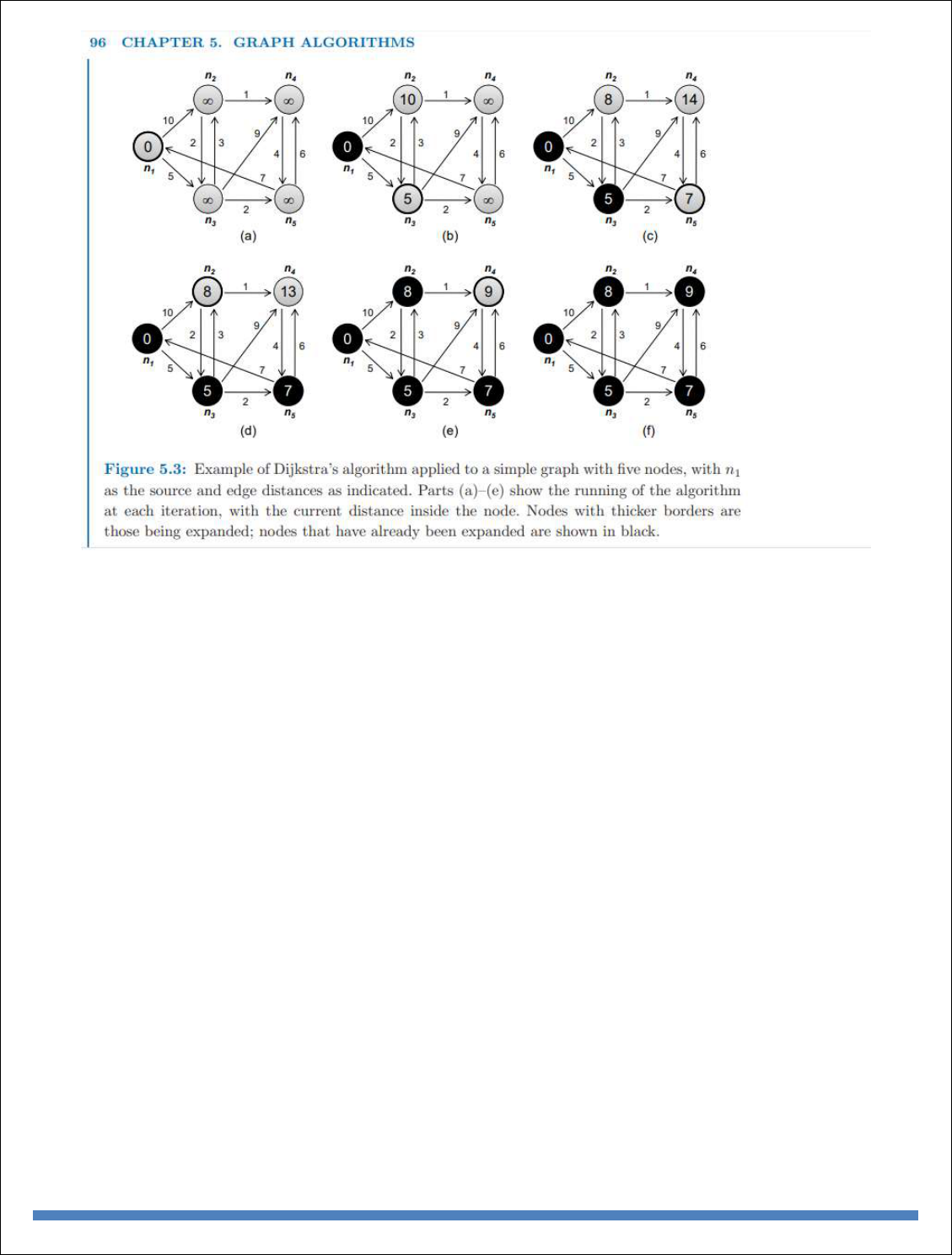
BIG DATA ANALYTICS
47
The key to Dijkstra’s algorithm is the priority queue that maintains a globallysorted list of nodes
by current distance. This is not possible in MapReduce, as the programming model does not
provide a mechanism for exchanging global data. Instead, we adopt a brute force approach known
as parallel breadth-first search. First, as a simplification let us assume that all edges have unit
distance (modeling, for example, hyperlinks on the web). This makes the algorithm easier to
understand, but we’ll relax this restriction later.
The intuition behind the algorithm is this: the distance of all nodes connected directly to the source
node is one; the distance of all nodes directly connected to those is two; and so on. Imagine water
rippling away from a rock dropped into a pond— that’s a good image of how parallel breadth-first
search works. However, what if there are multiple paths to the same node? Suppose we wish to
compute the shortest distance to node n. The shortest path must go through one of the nodes in M
that contains an outgoing edge to n: we need to examine all m ∈ M to find ms, the node with the
shortest distance. The shortest distance to n is the distance to ms plus one.
Pseudo-code for the implementation of the parallel breadth-first search algorithm is provided in
Figure 5.4. As with Dijkstra’s algorithm, we assume a connected, directed graph represented as
adjacency lists. Distance to each node is directly stored alongside the adjacency list of that node,
and initialized to ∞ for all nodes except for the source node. In the pseudo-code, we use n to denote
the node id (an integer) and N to denote the node’s corresponding data structure (adjacency list
and current distance). The algorithm works by mapping over all nodes and emitting a key-value
pair for each neighbor on the node’s adjacency list. The key contains the node id of the neighbor,
and the value is the current distance to the node plus one. This says: if we can reach node n with a
distance d, then we must be able to reach all the nodes that are connected to n with distance d + 1.

BIG DATA ANALYTICS
48
After shuffle and sort, reducers will receive keys corresponding to the destination node ids and
distances corresponding to all paths leading to that node. The reducer will select the shortest of
these distances and then update the distance in the node data structure.
h iteration corresponds to a MapReduce job. The first time we run the algorithm, we “discover”
all nodes that are connected to the source. The second iteration, we discover all nodes connected
to those, and so on. Each iteration of the algorithm expands the “search frontier” by one hop, and,
eventually, all nodes will be discovered with their shortest distances (assuming a fully-connected
graph). Before we discuss termination of the algorithm, there is one more detail required to make
the parallel breadth-first search algorithm work. We need to “pass along” the graph structure from
one iteration to the next. This is accomplished by emitting the node data structure itself, with the
node id as a key (Figure 5.4, line 4 in the mapper). In the reducer, we must distinguish the node
data structure from distance values (Figure 5.4, lines 5–6 in the reducer), and update the minimum
distance in the node data structure before emitting it as the final value. The final output is now
ready to serve as input to the next iteration.
So how many iterations are necessary to compute the shortest distance to all nodes? The answer is
the diameter of the graph, or the greatest distance between any pair of nodes. This number is
surprisingly small for many real-world problems: the saying “six degrees of separation” suggests
that everyone on the planet is connected to everyone else by at most six steps (the people a person
knows are one step away, people that they know are two steps away, etc.). If this is indeed true,
then parallel breadthfirst search on the global social network would take at most six MapReduce
iterations.
class Mapper
2: method Map(nid n, node N)
3: d ← N.Distance
4: Emit(nid n, N) . Pass along graph structure
5: for all nodeid m ∈ N.AdjacencyList do
6: Emit(nid m, d + 1) . Emit distances to reachable nodes
1: class Reducer
2: method Reduce(nid m, [d1, d2, . . .])
3: dmin ← ∞
4: M ← ∅
5: for all d ∈ counts [d1, d2, . . .] do
6: if IsNode(d) then
7: M ← d . Recover graph structure
8: else if d < dmin then . Look for shorter distance
9: dmin ← d
10: M.Distance ← dmin . Update shortest distance
11: Emit(nid m, node M)
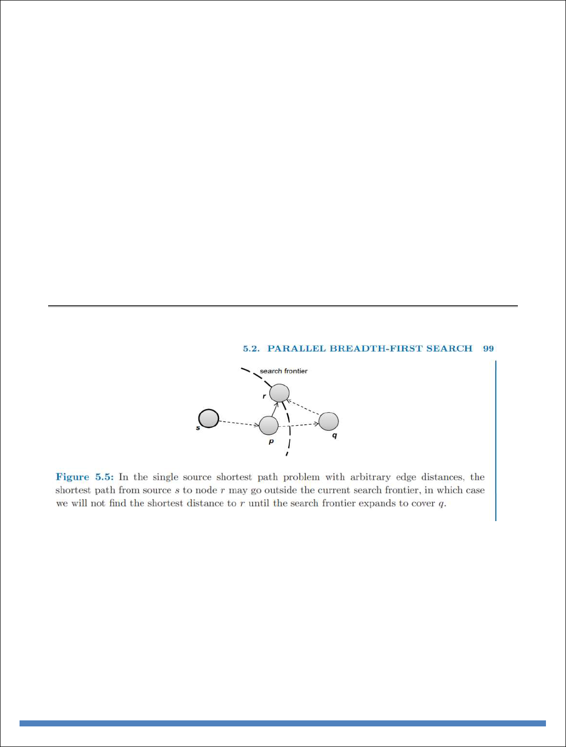
BIG DATA ANALYTICS
49
Figure 5.4: Pseudo-code for parallel breath-first search in MapReduce: the mappers emit distances
to reachable nodes, while the reducers select the minimum of those distances for each destination
node. Each iteration (one MapReduce job) of the algorithm expands the “search frontier” by one
hop.
For more serious academic studies of “small world” phenomena in networks, we refer the reader
to a number of publications [61, 62, 152, 2]. In practical terms, we iterate the algorithm until there
are no more node distances that are ∞. Since the graph is connected, all nodes are reachable, and
since all edge distances are one, all discovered nodes are guaranteed to have the shortest distances
(i.e., there is not a shorter path that goes through a node that hasn’t been discovered).
The actual checking of the termination condition must occur outside of MapReduce. Typically,
execution of an iterative MapReduce algorithm requires a nonMapReduce “driver” program,
which submits a MapReduce job to iterate the algorithm, checks to see if a termination condition
has been met, and if not, repeats. Hadoop provides a lightweight API for constructs called
“counters”, which, as the name suggests, can be used for counting events that occur during
execution, e.g., number of corrupt records, number of times a certain condition is met, or anything
that the programmer desires. Counters can be defined to count the number of nodes that have
distances of ∞: at the end of the job, the driver program can access the final counter value and
check to see if another iteration is necessary.
Finally, as with Dijkstra’s algorithm in the form presented earlier, the parallel breadth-first search
algorithm only finds the shortest distances, not the actual shortest paths. However, the path can be
straightforwardly recovered. Storing “backpointers” at each node, as with Dijkstra’s algorithm,
will work, but may not be efficient since the graph needs to be traversed again to reconstruct the
path segments. A simpler approach is to emit paths along with distances in the mapper, so that
each node will have its shortest path easily accessible at all times. The additional space
requirements for shuffling these data from mappers to reducers are relatively modest, since for the
most part paths (i.e., sequence of node ids) are relatively short.
Up until now, we have been assuming that all edges are unit distance. Let us relax that restriction
and see what changes are required in the parallel breadth-first search algorithm. The adjacency
lists, which were previously lists of node ids, must now encode the edge distances as well. In line

BIG DATA ANALYTICS
50
6 of the mapper code in Figure 5.4, instead of emitting d + 1 as the value, we must now emit d +
w where w is the edge distance. No other changes to the algorithm are required, but the termination
behavior is very different. To illustrate, consider the graph fragment in Figure 5.5, where s is the
source node, and in this iteration, we just “discovered” node r for the very first time. Assume for
the sake of argument that we’ve already discovered the shortest distance to node p, and that the
shortest distance to r so far goes through p. This, however, does not guarantee that we’ve
discovered the shortest distance to r, since there may exist a path going through q that we haven’t
encountered yet (because it lies outside the search frontier).6 However, as the search frontier
expands, we’ll eventually cover q and all other nodes along the path from p to q to r—which means
that with sufficient iterations, we will discover the shortest distance to r. But how do we know that
we’ve found the shortest distance to p? Well, if the shortest path to p lies within the search frontier,
we would have already discovered it. And if it doesn’t, the above argument applies. Similarly, we
can repeat the same argument for all nodes on the path from s to p. The conclusion is that, with
sufficient iterations, we’ll eventually discover all the shortest distances.
So exactly how many iterations does “eventually” mean? In the worst case, we might need as many
iterations as there are nodes in the graph minus one. In fact, it is not difficult to construct graphs
that will elicit this worse-case behavior: Figure 5.6 provides an example, with n1 as the source.
The parallel breadth-first search algorithm would not discover that the shortest path from n1 to n6
goes through n3, n4, and n5 until the fifth iteration. Three more iterations are necessary to cover
the rest of the graph. Fortunately, for most real-world graphs, such extreme cases are rare, and the
number of iterations necessary to discover all shortest distances is quite close to the diameter of
the graph, as in the unit edge distance case.
In practical terms, how do we know when to stop iterating in the case of arbitrary edge distances?
The algorithm can terminate when shortest distances at every node no longer change. Once again,
we can use counters to keep track of such events. Every time we encounter a shorter distance in
the reducer, we increment a counter. At the end of each MapReduce iteration, the driver program
reads the counter value and determines if another iteration is necessary.
Compared to Dijkstra’s algorithm on a single processor, parallel breadth-first search in
MapReduce can be characterized as a brute force approach that “wastes” a lot of time performing
computations whose results are discarded. At each iteration, the algorithm attempts to recompute
distances to all nodes, but in reality only useful work is done along the search frontier: inside the
search frontier, the algorithm is simply repeating previous computations.7 Outside the search
frontier, the algorithm hasn’t discovered any paths to nodes there yet, so no meaningful work is
done. Dijkstra’s algorithm, on the other hand, is far more efficient. Every time a node is explored,
we’re guaranteed to have already found the shortest path to it. However, this is made possible by
maintaining a global data structure (a priority queue) that holds nodes sorted by distance—this is
not possible in MapReduce because the programming model does not provide support for global
data that is mutable and accessible by the mappers and reducers. These inefficiencies represent the
cost of parallelization.
The parallel breadth-first search algorithm is instructive in that it represents the prototypical
structure of a large class of graph algorithms in MapReduce. They share in the following
characteristics:

BIG DATA ANALYTICS
51
The graph structure is represented with adjacency lists, which is part of some larger node
data structure that may contain additional information (variables to store intermediate output,
features of the nodes). In many cases, features are attached to edges as well (e.g., edge weights).
The graph structure is represented with adjacency lists, which is part of some larger node
data structure that may contain additional information (variables to store intermediate output,
features of the nodes). In many cases, features are attached to edges as well (e.g., edge weights).
In addition to computations, the graph itself is also passed from the mapper to the reducer.
In the reducer, the data structure corresponding to each node is updated and written back to disk.
Graph algorithms in MapReduce are generally iterative, where the output of the previous
iteration serves as input to the next iteration. The process is controlled by a non-MapReduce driver
program that checks for termination.
For parallel breadth-first search, the mapper computation is the current distance plus edge
distance (emitting distances to neighbors), while the reducer computation is the Min function
(selecting the shortest path). As we will see in the next section, the MapReduce algorithm for
PageRank works in much the same way

BIG DATA ANALYTICS
52
UNIT-IV
INTRODUCTION TO HIVE AND PIG
The term ‘Big Data’ is used for collections of large datasets that include huge volume, high
velocity, and a variety of data that is increasing day by day. Using traditional data management
systems, it is difficult to process Big Data. Therefore, the Apache Software Foundation introduced
a framework called Hadoop to solve Big Data management and processing challenges.
Hadoop
Hadoop is an open-source framework to store and process Big Data in a distributed environment.
It contains two modules, one is MapReduce and another is Hadoop Distributed File System
(HDFS).
MapReduce: It is a parallel programming model for processing large amounts of
structured, semi-structured, and unstructured data on large clusters of commodity
hardware.
HDFS:Hadoop Distributed File System is a part of Hadoop framework, used to store and
process the datasets. It provides a fault-tolerant file system to run on commodity hardware.
The Hadoop ecosystem contains different sub-projects (tools) such as Sqoop, Pig, and Hive that
are used to help Hadoop modules.
Sqoop: It is used to import and export data to and from between HDFS and RDBMS.
Pig: It is a procedural language platform used to develop a script for MapReduce
operations.
Hive: It is a platform used to develop SQL type scripts to do MapReduce operations.
Note: There are various ways to execute MapReduce operations:
The traditional approach using Java MapReduce program for structured, semi-structured,
and unstructured data.
The scripting approach for MapReduce to process structured and semi structured data using
Pig.
The Hive Query Language (HiveQL or HQL) for MapReduce to process structured data
using Hive.
What is Hive
Hive is a data warehouse infrastructure tool to process structured data in Hadoop. It resides on
top of Hadoop to summarize Big Data, and makes querying and analyzing easy.
Initially Hive was developed by Facebook, later the Apache Software Foundation took it up and
developed it further as an open source under the name Apache Hive. It is used by different
companies. For example, Amazon uses it in Amazon Elastic MapReduce.
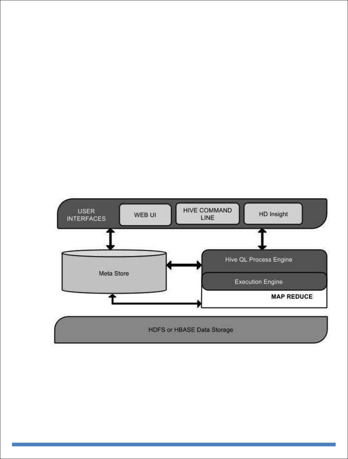
BIG DATA ANALYTICS
53
Hive is not
A relational database
A design for OnLine Transaction Processing (OLTP)
A language for real-time queries and row-level updates
Features of Hive
It stores schema in a database and processed data into HDFS.
It is designed for OLAP.
It provides SQL type language for querying called HiveQL or HQL.
It is familiar, fast, scalable, and extensible.
Architecture of Hive
The following component diagram depicts the architecture of Hive:
This component diagram contains different units. The following table describes each unit:
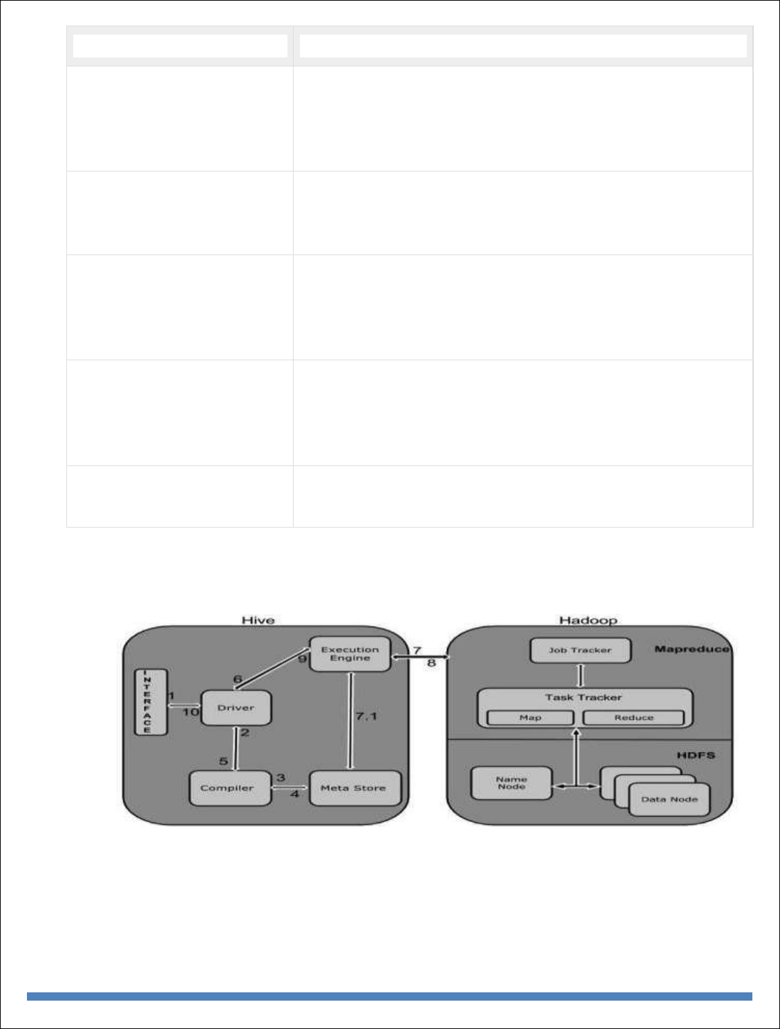
BIG DATA ANALYTICS
54
Unit Name
Operation
User Interface
Hive is a data warehouse infrastructure software that can
create interaction between user and HDFS. The user interfaces that
Hive supports are Hive Web UI, Hive command line, and Hive HD
Insight (In Windows server).
Meta Store
Hive chooses respective database servers to store the
schema or Metadata of tables, databases, columns in a table, their
data types, and HDFS mapping.
HiveQL Process Engine
HiveQL is similar to SQL for querying on schema info on
the Metastore. It is one of the replacements of traditional approach
for MapReduce program. Instead of writing MapReduce program
in Java, we can write a query for MapReduce job and process it.
Execution Engine
The conjunction part of HiveQL process Engine and
MapReduce is Hive Execution Engine. Execution engine processes
the query and generates results as same as MapReduce results. It
uses the flavor of MapReduce.
HDFS or HBASE
Hadoop distributed file system or HBASE are the data
storage techniques to store data into file system.
Working of Hive
The following diagram depicts the workflow between Hive and Hadoop.

BIG DATA ANALYTICS
55
The following table defines how Hive interacts with Hadoop framework:
Step
No.
Operation
1
Execute Query
The Hive interface such as Command Line or Web UI sends query to Driver (any database
driver such as JDBC, ODBC, etc.) to execute.
2
Get Plan
The driver takes the help of query compiler that parses the query to check the syntax and
query plan or the requirement of query.
3
Get Metadata
The compiler sends metadata request to Metastore (any database).
4
Send Metadata
Metastore sends metadata as a response to the compiler.
5
Send Plan
The compiler checks the requirement and resends the plan to the driver. Up to here, the
parsing and compiling of a query is complete.
6
Execute Plan
The driver sends the execute plan to the execution engine.
7
Execute Job
Internally, the process of execution job is a MapReduce job. The execution engine sends
the job to JobTracker, which is in Name node and it assigns this job to TaskTracker, which
is in Data node. Here, the query executes MapReduce job.
7.1
Metadata Ops

BIG DATA ANALYTICS
56
Meanwhile in execution, the execution engine can execute metadata operations with
Metastore.
8
Fetch Result
The execution engine receives the results from Data nodes.
9
Send Results
The execution engine sends those resultant values to the driver.
10
Send Results
The driver sends the results to Hive Interfaces.
File Formats in Hive
File Format specifies how records are encoded in files
Record Format implies how a stream of bytes for a given record are encoded
The default file format is TEXTFILE – each record is a line in the file
Hive uses different control characters as delimeters in textfiles
ᶺA ( octal 001) , ᶺB(octal 002), ᶺC(octal 003), \n
The term field is used when overriding the default delimiter
FIELDS TERMINATED BY ‘\001’
Supports text files – csv, tsv
TextFile can contain JSON or XML documents.
ommonly used File Formats –
1. TextFile format
Suitable for sharing data with other tools
Can be viewed/edited manually
2. SequenceFile
Flat files that stores binary key ,value pair
SequenceFile offers a Reader ,Writer, and Sorter classes for reading ,writing, and sorting
respectively
Supports – Uncompressed, Record compressed ( only value is compressed) and Block
compressed ( both key,value compressed) formats
3. RCFile
RCFile stores columns of a table in a record columnar way
4. ORC
5. AVRO

BIG DATA ANALYTICS
57
Hive Commands
Hive supports Data definition Language(DDL), Data Manipulation Language(DML) and User
defined functions.
Hive DDL Commands
create database
drop database
create table
drop table
alter table
create index
create view
Hive DML Commands
Select
Where
Group By
Order By
Load Data
Join:
o Inner Join
o Left Outer Join
o Right Outer Join
o Full Outer Join
Hive DDL Commands
Create Database Statement
A database in Hive is a namespace or a collection of tables.

BIG DATA ANALYTICS
58
1. hive> CREATE SCHEMA userdb;
2. hive> SHOW DATABASES;
Drop database
1. ive> DROP DATABASE IF EXISTS userdb;
Creating Hive Tables
Create a table called Sonoo with two columns, the first being an integer and the other a string.
1. hive> CREATE TABLE Sonoo(foo INT, bar STRING);
Create a table called HIVE_TABLE with two columns and a partition column called ds. The
partition column is a virtual column. It is not part of the data itself but is derived from the partition
that a particular dataset is loaded into.By default, tables are assumed to be of text input format and
the delimiters are assumed to be ^A(ctrl-a).
1. hive> CREATE TABLE HIVE_TABLE (foo INT, bar STRING) PARTITIONED BY (ds STRI
NG);
Browse the table
1. hive> Show tables;
Altering and Dropping Tables
1. hive> ALTER TABLE Sonoo RENAME TO Kafka;
2. hive> ALTER TABLE Kafka ADD COLUMNS (col INT);
3. hive> ALTER TABLE HIVE_TABLE ADD COLUMNS (col1 INT COMMENT 'a comment');
4. hive> ALTER TABLE HIVE_TABLE REPLACE COLUMNS (col2 INT, weight STRING, baz
INT COMMENT 'baz replaces new_col1');
Hive DML Commands
To understand the Hive DML commands, let's see the employee and employee_department table
first.
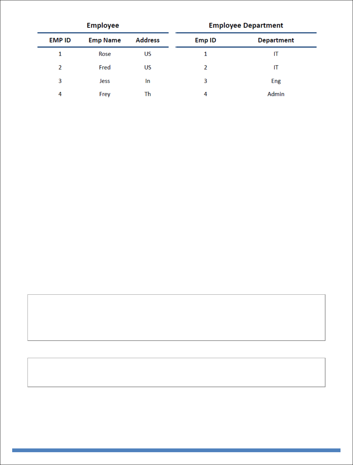
BIG DATA ANALYTICS
59
LOAD DATA
1. hive> LOAD DATA LOCAL INPATH './usr/Desktop/kv1.txt' OVERWRITE INTO TABLE Employe
e;
SELECTS and FILTERS
1. hive> SELECT E.EMP_ID FROM Employee E WHERE E.Address='US';
GROUP BY
1. hive> hive> SELECT E.EMP_ID FROM Employee E GROUP BY E.Addresss;
Adding a Partition
We can add partitions to a table by altering the table. Let us assume we have a table
called employee with fields such as Id, Name, Salary, Designation, Dept, and yoj.
Syntax:
ALTER TABLE table_name ADD [IF NOT EXISTS] PARTITION partition_spec
[LOCATION 'location1'] partition_spec [LOCATION 'location2'] ...;
partition_spec:
: (p_column = p_col_value, p_column = p_col_value, ...)
The following query is used to add a partition to the employee table.
hive> ALTER TABLE employee
> ADD PARTITION (year=’2012’)
> location '/2012/part2012';
Renaming a Partition
The syntax of this command is as follows.

BIG DATA ANALYTICS
60
ALTER TABLE table_name PARTITION partition_spec RENAME TO PARTITION
partition_spec;
The following query is used to rename a partition:
hive> ALTER TABLE employee PARTITION (year=’1203’)
> RENAME TO PARTITION (Yoj=’1203’);
Dropping a Partition
The following syntax is used to drop a partition:
ALTER TABLE table_name DROP [IF EXISTS] PARTITION partition_spec, PARTITION
partition_spec,...;
The following query is used to drop a partition:
hive> ALTER TABLE employee DROP [IF EXISTS]
> PARTITION (year=’1203’);
Hive Query Language
The Hive Query Language (HiveQL) is a query language for Hive to process and analyze
structured data in a Metastore. This chapter explains how to use the SELECT statement with
WHERE clause.
SELECT statement is used to retrieve the data from a table. WHERE clause works similar to a
condition. It filters the data using the condition and gives you a finite result. The built-in operators
and functions generate an expression, which fulfils the condition.
Syntax
Given below is the syntax of the SELECT query:
SELECT [ALL | DISTINCT] select_expr, select_expr, ...
FROM table_reference
[WHERE where_condition]
[GROUP BY col_list]
[HAVING having_condition]
[CLUSTER BY col_list | [DISTRIBUTE BY col_list] [SORT BY col_list]]
[LIMIT number];
Example
Let us take an example for SELECT…WHERE clause. Assume we have the employee table as
given below, with fields named Id, Name, Salary, Designation, and Dept. Generate a query to
retrieve the employee details who earn a salary of more than Rs 30000.

BIG DATA ANALYTICS
61
+------+--------------+-------------+-------------------+--------+
| ID | Name | Salary | Designation | Dept |
+------+--------------+-------------+-------------------+--------+
|1201 | Gopal | 45000 | Technical manager | TP |
|1202 | Manisha | 45000 | Proofreader | PR |
|1203 | Masthanvali | 40000 | Technical writer | TP |
|1204 | Krian | 40000 | Hr Admin | HR |
|1205 | Kranthi | 30000 | Op Admin | Admin |
+------+--------------+-------------+-------------------+--------+
The following query retrieves the employee details using the above scenario:
hive> SELECT * FROM employee WHERE salary>30000;
On successful execution of the query, you get to see the following response:
+------+--------------+-------------+-------------------+--------+
| ID | Name | Salary | Designation | Dept |
+------+--------------+-------------+-------------------+--------+
|1201 | Gopal | 45000 | Technical manager | TP |
|1202 | Manisha | 45000 | Proofreader | PR |
|1203 | Masthanvali | 40000 | Technical writer | TP |
|1204 | Krian | 40000 | Hr Admin | HR |
+------+--------------+-------------+-------------------+--------+
JDBC Program
The JDBC program to apply where clause for the given example is as follows.
import java.sql.SQLException;
import java.sql.Connection;
import java.sql.ResultSet;
import java.sql.Statement;
import java.sql.DriverManager;
public class HiveQLWhere {
private static String driverName = "org.apache.hadoop.hive.jdbc.HiveDriver";
public static void main(String[] args) throws SQLException {
// Register driver and create driver instance
Class.forName(driverName);
// get connection
Connection con = DriverManager.getConnection("jdbc:hive://localhost:10000/userdb", "",
"");
// create statement
Statement stmt = con.createStatement();
// execute statement

BIG DATA ANALYTICS
62
Resultset res = stmt.executeQuery("SELECT * FROM employee WHERE salary>30000;");
System.out.println("Result:");
System.out.println(" ID \t Name \t Salary \t Designation \t Dept ");
while (res.next()) {
System.out.println(res.getInt(1) + " " + res.getString(2) + " " + res.getDouble(3) + " " +
res.getString(4) + " " + res.getString(5));
}
con.close();
}
}
Save the program in a file named HiveQLWhere.java. Use the following commands to compile
and execute this program.
$ javac HiveQLWhere.java
$ java HiveQLWhere
Output:
ID Name Salary Designation Dept
1201 Gopal 45000 Technical manager TP
1202 Manisha 45000 Proofreader PR
1203 Masthanvali 40000 Technical writer TP
1204 Krian 40000 Hr Admin HR
The ORDER BY clause is used to retrieve the details based on one column and sort the result set
by ascending or descending order.
Syntax
Given below is the syntax of the ORDER BY clause:
SELECT [ALL | DISTINCT] select_expr, select_expr, ...
FROM table_reference
[WHERE where_condition]
[GROUP BY col_list]
[HAVING having_condition]
[ORDER BY col_list]]
[LIMIT number];

BIG DATA ANALYTICS
63
Example
Let us take an example for SELECT...ORDER BY clause. Assume employee table as given
below, with the fields named Id, Name, Salary, Designation, and Dept. Generate a query to
retrieve the employee details in order by using Department name.
+------+--------------+-------------+-------------------+--------+
| ID | Name | Salary | Designation | Dept |
+------+--------------+-------------+-------------------+--------+
|1201 | Gopal | 45000 | Technical manager | TP |
|1202 | Manisha | 45000 | Proofreader | PR |
|1203 | Masthanvali | 40000 | Technical writer | TP |
|1204 | Krian | 40000 | Hr Admin | HR |
|1205 | Kranthi | 30000 | Op Admin | Admin |
+------+--------------+-------------+-------------------+--------+
The following query retrieves the employee details using the above scenario:
hive> SELECT Id, Name, Dept FROM employee ORDER BY DEPT;
On successful execution of the query, you get to see the following response:
+------+--------------+-------------+-------------------+--------+
| ID | Name | Salary | Designation | Dept |
+------+--------------+-------------+-------------------+--------+
|1205 | Kranthi | 30000 | Op Admin | Admin |
|1204 | Krian | 40000 | Hr Admin | HR |
|1202 | Manisha | 45000 | Proofreader | PR |
|1201 | Gopal | 45000 | Technical manager | TP |
|1203 | Masthanvali | 40000 | Technical writer | TP |
+------+--------------+-------------+-------------------+--------+
JDBC Program
Here is the JDBC program to apply Order By clause for the given example.
import java.sql.SQLException;
import java.sql.Connection;
import java.sql.ResultSet;
import java.sql.Statement;
import java.sql.DriverManager;
public class HiveQLOrderBy {
private static String driverName = "org.apache.hadoop.hive.jdbc.HiveDriver";
public static void main(String[] args) throws SQLException {
// Register driver and create driver instance
Class.forName(driverName);
// get connection

BIG DATA ANALYTICS
64
Connection con = DriverManager.getConnection("jdbc:hive://localhost:10000/userdb", "",
"");
// create statement
Statement stmt = con.createStatement();
// execute statement
Resultset res = stmt.executeQuery("SELECT * FROM employee ORDER BY DEPT;");
System.out.println(" ID \t Name \t Salary \t Designation \t Dept ");
while (res.next()) {
System.out.println(res.getInt(1) + " " + res.getString(2) + " " + res.getDouble(3) + " " +
res.getString(4) + " " + res.getString(5));
}
con.close();
}
}
Save the program in a file named HiveQLOrderBy.java. Use the following commands to compile
and execute this program.
$ javac HiveQLOrderBy.java
$ java HiveQLOrderBy
Output:
ID Name Salary Designation Dept
1205 Kranthi 30000 Op Admin Admin
1204 Krian 40000 Hr Admin HR
1202 Manisha 45000 Proofreader PR
1201 Gopal 45000 Technical manager TP
1203 Masthanvali 40000 Technical writer TP
1204 Krian 40000 Hr Admin HR
The GROUP BY clause is used to group all the records in a result set using a particular collection
column. It is used to query a group of records.
Syntax
The syntax of GROUP BY clause is as follows:
SELECT [ALL | DISTINCT] select_expr, select_expr, ...
FROM table_reference
[WHERE where_condition]
[GROUP BY col_list]
[HAVING having_condition]
[ORDER BY col_list]]

BIG DATA ANALYTICS
65
[LIMIT number];
Example
Let us take an example of SELECT…GROUP BY clause. Assume employee table as given
below, with Id, Name, Salary, Designation, and Dept fields. Generate a query to retrieve the
number of employees in each department.
+------+--------------+-------------+-------------------+--------+
| ID | Name | Salary | Designation | Dept |
+------+--------------+-------------+-------------------+--------+
|1201 | Gopal | 45000 | Technical manager | TP |
|1202 | Manisha | 45000 | Proofreader | PR |
|1203 | Masthanvali | 40000 | Technical writer | TP |
|1204 | Krian | 45000 | Proofreader | PR |
|1205 | Kranthi | 30000 | Op Admin | Admin |
+------+--------------+-------------+-------------------+--------+
The following query retrieves the employee details using the above scenario.
hive> SELECT Dept,count(*) FROM employee GROUP BY DEPT;
On successful execution of the query, you get to see the following response:
+------+--------------+
| Dept | Count(*) |
+------+--------------+
|Admin | 1 |
|PR | 2 |
|TP | 3 |
+------+--------------+
JDBC Program
Given below is the JDBC program to apply the Group By clause for the given example.
import java.sql.SQLException;
import java.sql.Connection;
import java.sql.ResultSet;
import java.sql.Statement;
import java.sql.DriverManager;
public class HiveQLGroupBy {
private static String driverName = "org.apache.hadoop.hive.jdbc.HiveDriver";
public static void main(String[] args) throws SQLException {
// Register driver and create driver instance
Class.forName(driverName);
// get connection

BIG DATA ANALYTICS
66
Connection con = DriverManager.
getConnection("jdbc:hive://localhost:10000/userdb", "", "");
// create statement
Statement stmt = con.createStatement();
// execute statement
Resultset res = stmt.executeQuery(“SELECT Dept,count(*) ” + “FROM employee GROUP
BY DEPT; ”);
System.out.println(" Dept \t count(*)");
while (res.next()) {
System.out.println(res.getString(1) + " " + res.getInt(2));
}
con.close();
}
}
Save the program in a file named HiveQLGroupBy.java. Use the following commands to compile
and execute this program.
$ javac HiveQLGroupBy.java
$ java HiveQLGroupBy
Output:
Dept Count(*)
Admin 1
PR 2
TP 3
JOIN is a clause that is used for combining specific fields from two tables by using values
common to each one. It is used to combine records from two or more tables in the database.
Syntax
join_table:
table_reference JOIN table_factor [join_condition]
| table_reference {LEFT|RIGHT|FULL} [OUTER] JOIN table_reference
join_condition
| table_reference LEFT SEMI JOIN table_reference join_condition
| table_reference CROSS JOIN table_reference [join_condition]
Example
We will use the following two tables in this chapter. Consider the following table named
CUSTOMERS..

BIG DATA ANALYTICS
67
+----+----------+-----+-----------+----------+
| ID | NAME | AGE | ADDRESS | SALARY |
+----+----------+-----+-----------+----------+
| 1 | Ramesh | 32 | Ahmedabad | 2000.00 |
| 2 | Khilan | 25 | Delhi | 1500.00 |
| 3 | kaushik | 23 | Kota | 2000.00 |
| 4 | Chaitali | 25 | Mumbai | 6500.00 |
| 5 | Hardik | 27 | Bhopal | 8500.00 |
| 6 | Komal | 22 | MP | 4500.00 |
| 7 | Muffy | 24 | Indore | 10000.00 |
+----+----------+-----+-----------+----------+
Consider another table ORDERS as follows:
+-----+---------------------+-------------+--------+
|OID | DATE | CUSTOMER_ID | AMOUNT |
+-----+---------------------+-------------+--------+
| 102 | 2009-10-08 00:00:00 | 3 | 3000 |
| 100 | 2009-10-08 00:00:00 | 3 | 1500 |
| 101 | 2009-11-20 00:00:00 | 2 | 1560 |
| 103 | 2008-05-20 00:00:00 | 4 | 2060 |
+-----+---------------------+-------------+--------+
There are different types of joins given as follows:
JOIN
LEFT OUTER JOIN
RIGHT OUTER JOIN
FULL OUTER JOIN
JOIN
JOIN clause is used to combine and retrieve the records from multiple tables. JOIN is same as
OUTER JOIN in SQL. A JOIN condition is to be raised using the primary keys and foreign keys
of the tables.
The following query executes JOIN on the CUSTOMER and ORDER tables, and retrieves the
records:
hive> SELECT c.ID, c.NAME, c.AGE, o.AMOUNT
FROM CUSTOMERS c JOIN ORDERS o
ON (c.ID = o.CUSTOMER_ID);
On successful execution of the query, you get to see the following response:
+----+----------+-----+--------+
| ID | NAME | AGE | AMOUNT |
+----+----------+-----+--------+
| 3 | kaushik | 23 | 3000 |
| 3 | kaushik | 23 | 1500 |
| 2 | Khilan | 25 | 1560 |

BIG DATA ANALYTICS
68
| 4 | Chaitali | 25 | 2060 |
+----+----------+-----+--------+
LEFT OUTER JOIN
The HiveQL LEFT OUTER JOIN returns all the rows from the left table, even if there are no
matches in the right table. This means, if the ON clause matches 0 (zero) records in the right table,
the JOIN still returns a row in the result, but with NULL in each column from the right table.
A LEFT JOIN returns all the values from the left table, plus the matched values from the right
table, or NULL in case of no matching JOIN predicate.
The following query demonstrates LEFT OUTER JOIN between CUSTOMER and ORDER
tables:
hive> SELECT c.ID, c.NAME, o.AMOUNT, o.DATE
FROM CUSTOMERS c
LEFT OUTER JOIN ORDERS o
ON (c.ID = o.CUSTOMER_ID);
On successful execution of the query, you get to see the following response:
+----+----------+--------+---------------------+
| ID | NAME | AMOUNT | DATE |
+----+----------+--------+---------------------+
| 1 | Ramesh | NULL | NULL |
| 2 | Khilan | 1560 | 2009-11-20 00:00:00 |
| 3 | kaushik | 3000 | 2009-10-08 00:00:00 |
| 3 | kaushik | 1500 | 2009-10-08 00:00:00 |
| 4 | Chaitali | 2060 | 2008-05-20 00:00:00 |
| 5 | Hardik | NULL | NULL |
| 6 | Komal | NULL | NULL |
| 7 | Muffy | NULL | NULL |
+----+----------+--------+---------------------+
RIGHT OUTER JOIN
The HiveQL RIGHT OUTER JOIN returns all the rows from the right table, even if there are no
matches in the left table. If the ON clause matches 0 (zero) records in the left table, the JOIN still
returns a row in the result, but with NULL in each column from the left table.
A RIGHT JOIN returns all the values from the right table, plus the matched values from the left
table, or NULL in case of no matching join predicate.
The following query demonstrates RIGHT OUTER JOIN between the CUSTOMER and ORDER
tables.
notranslate"> hive> SELECT c.ID, c.NAME, o.AMOUNT, o.DATE FROM CUSTOMERS c
RIGHT OUTER JOIN ORDERS o ON (c.ID = o.CUSTOMER_ID);
On successful execution of the query, you get to see the following response:
+------+----------+--------+---------------------+

BIG DATA ANALYTICS
69
| ID | NAME | AMOUNT | DATE |
+------+----------+--------+---------------------+
| 3 | kaushik | 3000 | 2009-10-08 00:00:00 |
| 3 | kaushik | 1500 | 2009-10-08 00:00:00 |
| 2 | Khilan | 1560 | 2009-11-20 00:00:00 |
| 4 | Chaitali | 2060 | 2008-05-20 00:00:00 |
+------+----------+--------+---------------------+
FULL OUTER JOIN
The HiveQL FULL OUTER JOIN combines the records of both the left and the right outer tables
that fulfil the JOIN condition. The joined table contains either all the records from both the tables,
or fills in NULL values for missing matches on either side.
The following query demonstrates FULL OUTER JOIN between CUSTOMER and ORDER
tables:
hive> SELECT c.ID, c.NAME, o.AMOUNT, o.DATE
FROM CUSTOMERS c
FULL OUTER JOIN ORDERS o
ON (c.ID = o.CUSTOMER_ID);
On successful execution of the query, you get to see the following response:
+------+----------+--------+---------------------+
| ID | NAME | AMOUNT | DATE |
+------+----------+--------+---------------------+
| 1 | Ramesh | NULL | NULL |
| 2 | Khilan | 1560 | 2009-11-20 00:00:00 |
| 3 | kaushik | 3000 | 2009-10-08 00:00:00 |
| 3 | kaushik | 1500 | 2009-10-08 00:00:00 |
| 4 | Chaitali | 2060 | 2008-05-20 00:00:00 |
| 5 | Hardik | NULL | NULL |
| 6 | Komal | NULL | NULL |
| 7 | Muffy | NULL | NULL |
| 3 | kaushik | 3000 | 2009-10-08 00:00:00 |
| 3 | kaushik | 1500 | 2009-10-08 00:00:00 |
| 2 | Khilan | 1560 | 2009-11-20 00:00:00 |
| 4 | Chaitali | 2060 | 2008-05-20 00:00:00 |
+------+----------+--------+---------------------+
Bucketing #
•Bucketing concept is based on (hashing function on the bucketed column) mod (by total number
of buckets). The hash_function depends on the type of the bucketing column.
•Records with the same bucketed column will always be stored in the same bucket.
•We use CLUSTERED BY clause to divide the table into buckets.

BIG DATA ANALYTICS
70
•Physically, each bucket is just a file in the table directory, and Bucket numbering is 1-based.
•Bucketing can be done along with Partitioning on Hive tables and even without partitioning.
•Bucketed tables will create almost equally distributed data file parts, unless there is skew in data.
•Bucketing is enabled by setting hive.enforce.bucketing= true;
Advantages
•Bucketed tables offer efficient sampling than by non-bucketed tables. With sampling, we can try
out queries on a fraction of data for testing and debugging purpose when the original data sets are
very huge.
•As the data files are equal sized parts, map-side joins will be faster on bucketed tables than non-
bucketed tables.
•Bucketing concept also provides the flexibility to keep the records in each bucket to be sorted by
one or more columns. This makes map-side joins even more efficient, since the join of each bucket
becomes an efficient merge-sort.
Bucketing Vs Partitioning
•Partitioning helps in elimination of data, if used in WHERE clause, where as bucketing helps in
organizing data in each partition into multiple files, so that the same set of data is always written
in same bucket.
•Bucketing helps a lot in joining of columns.
•Hive Bucket is nothing but another technique of decomposing data or decreasing the data into
more manageable parts or equal parts.
Sampling
•TABLESAMPLE() gives more disordered and random records from a table as compared to
LIMIT. •We can sample using the rand() function, which returns a random number.
SELECT * from users TABLESAMPLE(BUCKET 3 OUT OF 10 ON rand()) s;
SELECT * from users TABLESAMPLE(BUCKET 3 OUT OF 10 ON rand()) s;
•Here rand() refers to any random column. •The denominator in the bucket clause represents the
number of buckets into which data will be hashed. •The numerator is the bucket number selected.
SELECT * from users TABLESAMPLE(BUCKET 2 OUT OF 4 ON name) s;
•If the columns specified in the TABLESAMPLE clause match the columns in the CLUSTERED
BY clause, TABLESAMPLE queries only scan the required hash partitions of the table.
SELECT * FROM buck_users TABLESAMPLE(BUCKET 1 OUT OF 2 ON id) s LIMIT 1;

BIG DATA ANALYTICS
71
Joins and Types #
Reduce-Side Join
•If datasets are large, reduce side join takes place.
Map-Side Join
•In case one of the dataset is small, map side join takes place. •In map side join, a local job runs to
create hash-table from content of HDFS file and sends it to every node.
SET hive.auto.convert.join =true;
Bucket Map Join
•The data must be bucketed on the keys used in the ON clause and the number of buckets for one
table must be a multiple of the number of buckets for the other table. •When these conditions are
met, Hive can join individual buckets between tables in the map phase, because it does not have
to fetch the entire content of one table to match against each bucket in the other table. •set
hive.optimize.bucketmapjoin =true; •SET hive.auto.convert.join =true;
SMBM Join
•Sort-Merge-Bucket (SMB) joins can be converted to SMB map joins as well.
•SMB joins are used wherever the tables are sorted and bucketed.
•The join boils down to just merging the already sorted tables, allowing this operation to be faster
than an ordinary map-join.
•set hive.enforce.sortmergebucketmapjoin =false;
•set hive.auto.convert.sortmerge.join =true;
•set hive.optimize.bucketmapjoin = true;
•set hive.optimize.bucketmapjoin.sortedmerge = true;
LEFT SEMI JOIN
•A left semi-join returns records from the lefthand table if records are found in the righthand table
that satisfy the ON predicates.
•It’s a special, optimized case of the more general inner join.
•Most SQL dialects support an IN … EXISTS construct to do the same thing.
•SELECT and WHERE clauses can’t reference columns from the righthand table.
•Right semi-joins are not supported in Hive.

BIG DATA ANALYTICS
72
•The reason semi-joins are more efficient than the more general inner join is as follows:
•For a given record in the lefthand table, Hive can stop looking for matching records in the
righthand table as soon as any match is found.
•At that point, the selected columns from the lefthand table record can be projected
•A file format is a way in which information is stored or encoded in a computer file.
•In Hive it refers to how records are stored inside the file.
•InputFormat reads key-value pairs from files.
•As we are dealing with structured data, each record has to be its own structure.
•How records are encoded in a file defines a file format.
•These file formats mainly vary between data encoding, compression rate, usage of space and disk
I/O.
•Hive does not verify whether the data that you are loading matches the schema for the table or
not. •However, it verifies if the file format matches the table definition or not.
SerDe in Hive #
•The SerDe interface allows you to instruct Hive as to how a record should be processed.
•A SerDe is a combination of a Serializer and a Deserializer (hence, Ser-De).
•The Deserializer interface takes a string or binary representation of a record, and translates it into
a Java object that Hive can manipulate.
•The Serializer, however, will take a Java object that Hive has been working with, and turn it into
something that Hive can write to HDFS or another supported system.
•Commonly, Deserializers are used at query time to execute SELECT statements, and Serializers
are used when writing data, such as through an INSERT-SELECT statement.
CSVSerDe
•Use ROW FORMAT SERDE ‘org.apache.hadoop.hive.serde2.OpenCSVSerde’
•Define following in SERDEPROPERTIES
( " separatorChar " = < value_of_separator
, " quoteChar " = < value_of_quote_character ,
" escapeChar “ = < value_of_escape_character

BIG DATA ANALYTICS
73
)
JSONSerDe
•Include hive-hcatalog-core-0.14.0.jar •Use ROW FORMAT SERDE ’
org.apache.hive.hcatalog.data.JsonSerDe ’
RegexSerDe
•It is used in case of pattern matching. •Use ROW FORMAT SERDE
'org.apache.hadoop.hive.contrib.serde2.RegexSerDe‘
•In SERDEPROPERTIES, define input pattern and output fields.
For Example
•input.regex = ‘(.)/(.)@(.*)’ •output.format.string’ = ’ 1 s 2 s 3 s’;
USE PARTITIONING AND BUCKETING
•Partitioning a table stores data in sub-directories categorized by table location, which allows Hive
to exclude unnecessary data from queries without reading all the data every time a new query is
made.
•Hive does support Dynamic Partitioning (DP) where column values are only known at
EXECUTION TIME. To enable Dynamic Partitioning :
SET hive.exec.dynamic.partition =true;
•Another situation we want to protect against dynamic partition insert is that the user may
accidentally specify all partitions to be dynamic partitions without specifying one static partition,
while the original intention is to just overwrite the sub-partitions of one root partition.
SET hive.exec.dynamic.partition.mode =strict;
To enable bucketing:
SET hive.enforce.bucketing =true;
Optimizations in Hive #
•Use Denormalisation , Filtering and Projection as early as possible to reduce data before join.
•Join is a costly affair and requires extra map-reduce phase to accomplish query job. With De-
normalisation, the data is present in the same table so there is no need for any joins, hence the
selects are very fast.

BIG DATA ANALYTICS
74
•As join requires data to be shuffled across nodes, use filtering and projection as early as possible
to reduce data before join.
TUNE CONFIGURATIONS
•To increase number of mapper, reduce split size :
SET mapred.max.split.size =1000000; (~1 MB)
•Compress map/reduce output
SET mapred.compress.map.output =true;
SET mapred.output.compress =true;
•Parallel execution
•Applies to MapReduce jobs that can run in parallel, for example jobs processing different source
tables before a join.
SET hive.exec.parallel =true;
USE ORCFILE
•Hive supports ORCfile , a new table storage format that sports fantastic speed improvements
through techniques like predicate push-down, compression and more.
•Using ORCFile for every HIVE table is extremely beneficial to get fast response times for your
HIVE queries.
USE TEZ
•With Hadoop2 and Tez , the cost of job submission and scheduling is minimized.
•Also Tez does not restrict the job to be only Map followed by Reduce; this implies that all the
query execution can be done in a single job without having to cross job boundaries.
•Let’s look at an example. Consider a click-stream event table:
CREATE TABLE clicks (
timestamp date,
sessionID string,
url string,
source_ip string
)
STORED as ORC
tblproperties (“ orc.compress ” = “SNAPPY”);
•Each record represents a click event, and we would like to find the latest URL for each sessionID
• One might consider the following approach:

BIG DATA ANALYTICS
75
SELECT clicks.sessionID, clicks.url FROM clicks inner join (select sessionID, max(timestamp)
as max_ts from clicks group by sessionID) latest ON clicks.sessionID = latest.sessionID and
clicks.timestamp = latest.max_ts;
•In the above query, we build a sub-query to collect the timestamp of the latest event in each
session, and then use an inner join to filter out the rest.
•While the query is a reasonable solution —from a functional point of view— it turns out there’s
a better way to re-write this query as follows:
SELECT ranked_clicks.sessionID , ranked_clicks.url FROM (SELECT sessionID , url , RANK()
over (partition by sessionID,order by timestamp desc ) as rank FROM clicks) ranked_clicks
WHERE ranked_clicks.rank =1;
•Here, we use Hive’s OLAP functionality (OVER and RANK) to achieve the same thing, but
without a Join.
•Clearly, removing an unnecessary join will almost always result in better performance, and when
using big data this is more important than ever.
MAKING MULTIPLE PASS OVER SAME DATA
•Hive has a special syntax for producing multiple aggregations from a single pass through a source
of data, rather than rescanning it for each aggregation.
•This change can save considerable processing time for large input data sets.
•For example, each of the following two queries creates a table from the same source table, history:
INSERT OVERWRITE TABLE sales
SELECT * FROM history WHERE action=‘purchased’;
INSERT OVERWRITE TABLE credits
SELECT * FROM history WHERE action=‘returned’;
Optimizations in Hive
•This syntax is correct, but inefficient.
•The following rewrite achieves the same thing, but using a single pass through the source history
table:
FROM history
INSERT OVERWRITE sales SELECT * WHERE action=‘purchased’
INSERT OVERWRITE credits SELECT * WHERE action=‘returned’;

BIG DATA ANALYTICS
76
What is Apache Pig
Apache Pig is a high-level data flow platform for executing MapReduce programs of Hadoop. The
language used for Pig is Pig Latin.
The Pig scripts get internally converted to Map Reduce jobs and get executed on data stored in
HDFS. Apart from that, Pig can also execute its job in Apache Tez or Apache Spark.
Pig can handle any type of data, i.e., structured, semi-structured or unstructured and stores the
corresponding results into Hadoop Data File System. Every task which can be achieved using PIG
can also be achieved using java used in MapReduce.
Features of Apache Pig
Let's see the various uses of Pig technology.
1) Ease of programming
Writing complex java programs for map reduce is quite tough for non-programmers. Pig makes
this process easy. In the Pig, the queries are converted to MapReduce internally.
2) Optimization opportunities
It is how tasks are encoded permits the system to optimize their execution automatically, allowing
the user to focus on semantics rather than efficiency.
3) Extensibility
A user-defined function is written in which the user can write their logic to execute over the data
set.
4) Flexible
It can easily handle structured as well as unstructured data.
5) In-built operators
It contains various type of operators such as sort, filter and joins.
Differences between Apache MapReduce and PIG
Advantages of Apache Pig
o Less code - The Pig consumes less line of code to perform any operation.
o Reusability - The Pig code is flexible enough to reuse again.

BIG DATA ANALYTICS
77
o Nested data types - The Pig provides a useful concept of nested data types like tuple, bag,
and map.
Pig Latin
The Pig Latin is a data flow language used by Apache Pig to analyze the data in Hadoop. It is a
textual language that abstracts the programming from the Java MapReduce idiom into a notation.
Pig Latin Statements
The Pig Latin statements are used to process the data. It is an operator that accepts a relation as an
input and generates another relation as an output.
o It can span multiple lines.
o Each statement must end with a semi-colon.
o It may include expression and schemas.
o By default, these statements are processed using multi-query execution
Pig Latin Conventions
Convention
Description
( )
The parenthesis can enclose one or more items. It can also be used to indicate
the tuple data type.
Example - (10, xyz, (3,6,9))
[ ]
The straight brackets can enclose one or more items. It can also be used to
indicate the map data type.
Example - [INNER | OUTER]
{ }
The curly brackets enclose two or more items. It can also be used to indicate
the bag data type
Example - { block | nested_block }
...
The horizontal ellipsis points indicate that you can repeat a portion of the code.
Example - cat path [path ...]
BIG DATA ANALYTICS
78
Latin Data Types
Simple Data Types
Type
Description
int
It defines the signed 32-bit integer.
Example - 2
long
It defines the signed 64-bit integer.
Example - 2L or 2l
float
It defines 32-bit floating point number.
Example - 2.5F or 2.5f or 2.5e2f or 2.5.E2F
double
It defines 64-bit floating point number.
Example - 2.5 or 2.5 or 2.5e2f or 2.5.E2F
chararray
It defines character array in Unicode UTF-8 format.
Example - javatpoint
bytearray
It defines the byte array.
boolean
It defines the boolean type values.
Example - true/false
datetime
It defines the values in datetime order.
Example - 1970-01- 01T00:00:00.000+00:00
biginteger
It defines Java BigInteger values.
Example - 5000000000000
bigdecimal
It defines Java BigDecimal values.
Example - 52.232344535345

BIG DATA ANALYTICS
79
Pig Data Types
Apache Pig supports many data types. A list of Apache Pig Data Types with description and
examples are given below.
Type
Description
Example
Int
Signed 32 bit integer
2
Long
Signed 64 bit integer
15L or 15l
Float
32 bit floating point
2.5f or 2.5F
Double
32 bit floating point
1.5 or 1.5e2 or
1.5E2
charArray
Character array
hello javatpoint
byteArray
BLOB(Byte array)
tuple
Ordered set of fields
(12,43)
bag
Collection f tuples
{(12,43),(54,28)}
map
collection of tuples
[open#apache]
Apache Pig Execution Modes
You can run Apache Pig in two modes, namely, Local Mode and HDFS mode.
Local Mode
In this mode, all the files are installed and run from your local host and local file system. There
is no need of Hadoop or HDFS. This mode is generally used for testing purpose.
MapReduce Mode
MapReduce mode is where we load or process the data that exists in the Hadoop File System
(HDFS) using Apache Pig. In this mode, whenever we execute the Pig Latin statements to process
the data, a MapReduce job is invoked in the back-end to perform a particular operation on the
data that exists in the HDFS.
Apache Pig Execution Mechanisms

BIG DATA ANALYTICS
80
Apache Pig scripts can be executed in three ways, namely, interactive mode, batch mode, and
embedded mode.
Interactive Mode (Grunt shell) − You can run Apache Pig in interactive mode using the
Grunt shell. In this shell, you can enter the Pig Latin statements and get the output (using
Dump operator).
Batch Mode (Script) − You can run Apache Pig in Batch mode by writing the Pig Latin
script in a single file with .pig extension.
Embedded Mode (UDF) − Apache Pig provides the provision of defining our own
functions (User Defined Functions) in programming languages such as Java, and using
them in our script.
Given below in the table are some frequently used Pig Commands.
Command
Function
load
Reads data from the system
Store
Writes data to file system
foreach
Applies expressions to each record and outputs one or more records
filter
Applies predicate and removes records that do not return true

BIG DATA ANALYTICS
81
Group/cogroup
Collects records with the same key from one or more inputs
join
Joins two or more inputs based on a key
order
Sorts records based on a key
distinct
Removes duplicate records
union
Merges data sets
split
Splits data into two or more sets based on filter conditions
stream
Sends all records through a user-provided binary
dump
Writes output to stdout

BIG DATA ANALYTICS
82
limit
Limits the number of records
Complex Types
Type
Description
tuple
It defines an ordered set of fields.
Example - (15,12)
bag
It defines a collection of tuples.
Example - {(15,12), (12,15)}
map
It defines a set of key-value pairs.
Example - [open#apache]
Pig Latin – Relational Operations
The following table describes the relational operators of Pig Latin.
Operator
Description
Loading and Storing
LOAD
To Load the data from the file system (local/HDFS) into a relation.
STORE
To save a relation to the file system (local/HDFS).
Filtering
BIG DATA ANALYTICS
83
FILTER
To remove unwanted rows from a relation.
DISTINCT
To remove duplicate rows from a relation.
FOREACH,
GENERATE
To generate data transformations based on columns of data.
STREAM
To transform a relation using an external program.
Grouping and Joining
JOIN
To join two or more relations.
COGROUP
To group the data in two or more relations.
GROUP
To group the data in a single relation.
CROSS
To create the cross product of two or more relations.
Sorting
ORDER
To arrange a relation in a sorted order based on one or more fields
(ascending or descending).
LIMIT
To get a limited number of tuples from a relation.
Combining and Splitting
UNION
To combine two or more relations into a single relation.
SPLIT
To split a single relation into two or more relations.

BIG DATA ANALYTICS
84
Diagnostic Operators
DUMP
To print the contents of a relation on the console.
DESCRIBE
To describe the schema of a relation.
EXPLAIN
To view the logical, physical, or MapReduce execution plans to compute
a relation.
ILLUSTRATE
To view the step-by-step execution of a series of statements.
Eval Functions
Given below is the list of eval functions provided by Apache Pig.
S.N.
Function & Description
1
AVG()
To compute the average of the numerical values within a bag.
2
BagToString()
To concatenate the elements of a bag into a string. While concatenating, we can place a
delimiter between these values (optional).
3
CONCAT()
To concatenate two or more expressions of same type.
4
COUNT()
To get the number of elements in a bag, while counting the number of tuples in a bag.
5
COUNT_STAR()

BIG DATA ANALYTICS
85
It is similar to the COUNT() function. It is used to get the number of elements in a bag.
6
DIFF()
To compare two bags (fields) in a tuple.
7
IsEmpty()
To check if a bag or map is empty.
8
MAX()
To calculate the highest value for a column (numeric values or chararrays) in a single-column
bag.
9
MIN()
To get the minimum (lowest) value (numeric or chararray) for a certain column in a single-
column bag.
10
PluckTuple()
Using the Pig Latin PluckTuple() function, we can define a string Prefix and filter the
columns in a relation that begin with the given prefix.
11
SIZE()
To compute the number of elements based on any Pig data type.
12
SUBTRACT()
To subtract two bags. It takes two bags as inputs and returns a bag which contains the tuples
of the first bag that are not in the second bag.
13
SUM()
To get the total of the numeric values of a column in a single-column bag.
14
TOKENIZE()
To split a string (which contains a group of words) in a single tuple and return a bag which
contains the output of the split operation.

BIG DATA ANALYTICS
86
Apache Pig provides extensive support for User Defined Functions (UDF’s). Using these UDF’s,
we can define our own functions and use them. The UDF support is provided in six programming
languages, namely, Java, Jython, Python, JavaScript, Ruby and Groovy.
For writing UDF’s, complete support is provided in Java and limited support is provided in all
the remaining languages. Using Java, you can write UDF’s involving all parts of the processing
like data load/store, column transformation, and aggregation. Since Apache Pig has been written
in Java, the UDF’s written using Java language work efficiently compared to other languages.
In Apache Pig, we also have a Java repository for UDF’s named Piggybank. Using Piggybank,
we can access Java UDF’s written by other users, and contribute our own UDF’s.
Types of UDF’s in Java
While writing UDF’s using Java, we can create and use the following three types of functions −
Filter Functions − The filter functions are used as conditions in filter statements. These
functions accept a Pig value as input and return a Boolean value.
Eval Functions − The Eval functions are used in FOREACH-GENERATE statements.
These functions accept a Pig value as input and return a Pig result.
Algebraic Functions − The Algebraic functions act on inner bags in a
FOREACHGENERATE statement. These functions are used to perform full MapReduce
operations on an inner bag.
Writing UDF’s using Java
To write a UDF using Java, we have to integrate the jar file Pig-0.15.0.jar. In this section, we
discuss how to write a sample UDF using Eclipse. Before proceeding further, make sure you have
installed Eclipse and Maven in your system.
Follow the steps given below to write a UDF function −
Open Eclipse and create a new project (say myproject).
Convert the newly created project into a Maven project.
Copy the following content in the pom.xml. This file contains the Maven dependencies for
Apache Pig and Hadoop-core jar files.
<project xmlns = "http://maven.apache.org/POM/4.0.0"
xmlns:xsi = "http://www.w3.org/2001/XMLSchema-instance"
xsi:schemaLocation = "http://maven.apache.org/POM/4.0.0http://maven.apache
.org/xsd/maven-4.0.0.xsd">
<modelVersion>4.0.0</modelVersion>
<groupId>Pig_Udf</groupId>
<artifactId>Pig_Udf</artifactId>
<version>0.0.1-SNAPSHOT</version>
<build>
<sourceDirectory>src</sourceDirectory>

BIG DATA ANALYTICS
87
<plugins>
<plugin>
<artifactId>maven-compiler-plugin</artifactId>
<version>3.3</version>
<configuration>
<source>1.7</source>
<target>1.7</target>
</configuration>
</plugin>
</plugins>
</build>
<dependencies>
<dependency>
<groupId>org.apache.pig</groupId>
<artifactId>pig</artifactId>
<version>0.15.0</version>
</dependency>
<dependency>
<groupId>org.apache.hadoop</groupId>
<artifactId>hadoop-core</artifactId>
<version>0.20.2</version>
</dependency>
</dependencies>
</project>
Save the file and refresh it. In the Maven Dependencies section, you can find the
downloaded jar files.
Create a new class file with name Sample_Eval and copy the following content in it.
import java.io.IOException;
import org.apache.pig.EvalFunc;
import org.apache.pig.data.Tuple;
import java.io.IOException;
import org.apache.pig.EvalFunc;
import org.apache.pig.data.Tuple;
public class Sample_Eval extends EvalFunc<String>{
public String exec(Tuple input) throws IOException {
if (input == null || input.size() == 0)
return null;
String str = (String)input.get(0);
return str.toUpperCase();
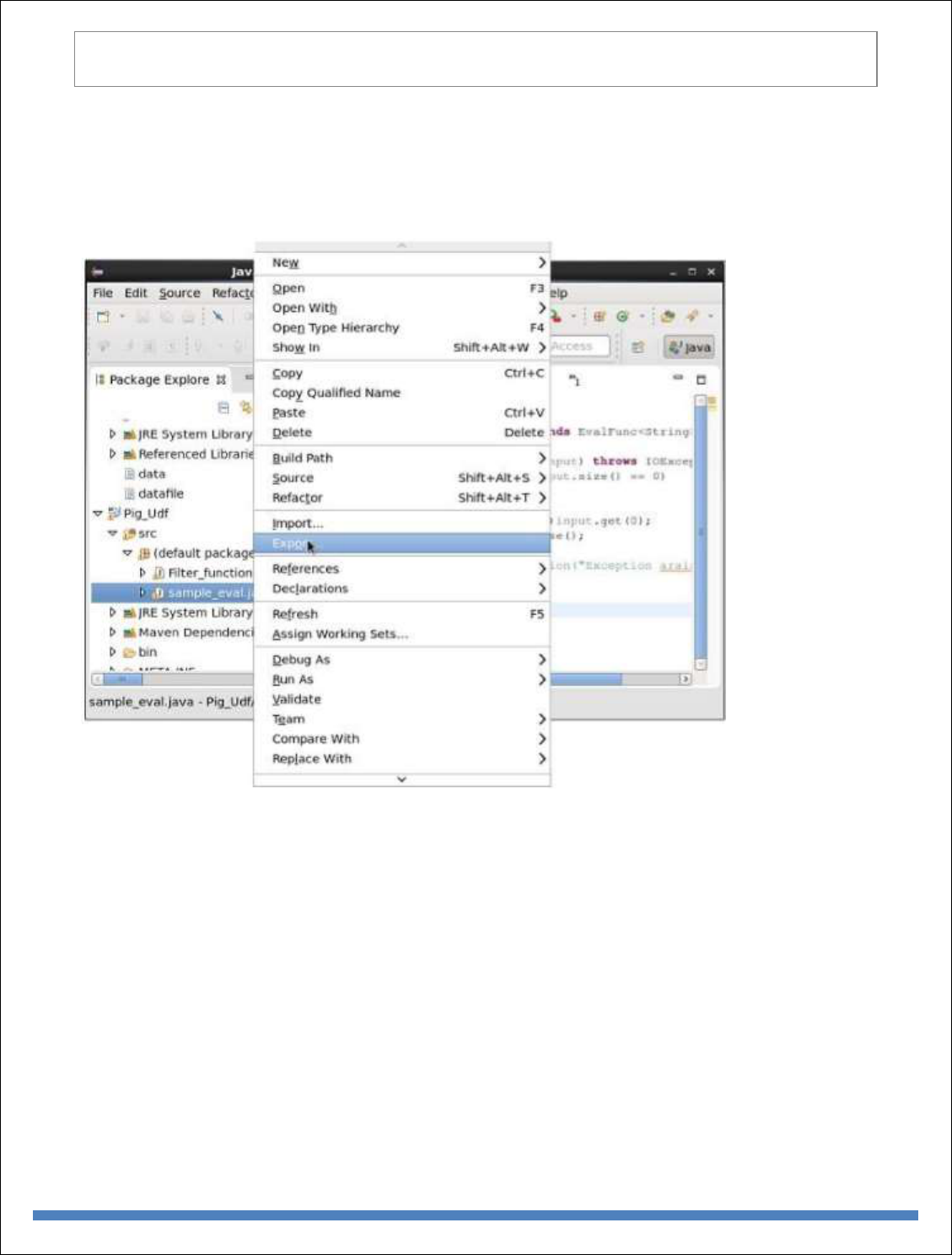
BIG DATA ANALYTICS
88
}
}
While writing UDF’s, it is mandatory to inherit the EvalFunc class and provide implementation
to exec() function. Within this function, the code required for the UDF is written. In the above
example, we have return the code to convert the contents of the given column to uppercase.
After compiling the class without errors, right-click on the Sample_Eval.java file. It gives
you a menu. Select export as shown in the following screenshot.
On clicking export, you will get the following window. Click on JAR file.
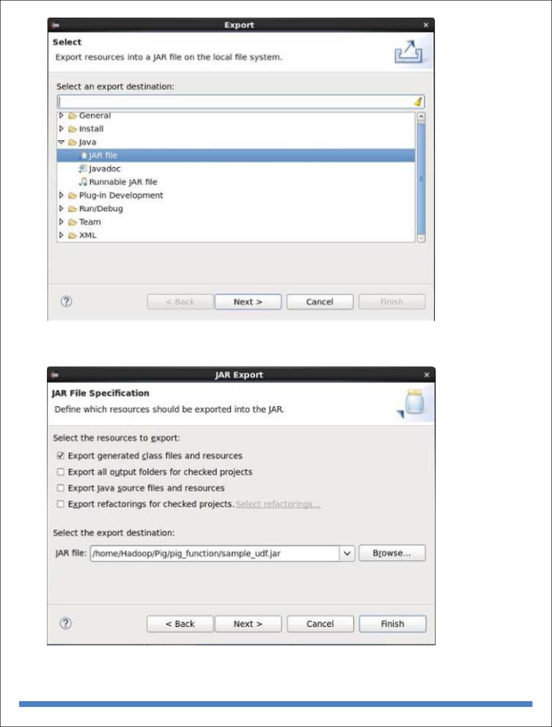
BIG DATA ANALYTICS
89
Proceed further by clicking Next> button. You will get another window where you need
to enter the path in the local file system, where you need to store the jar file.

BIG DATA ANALYTICS
90
Finally click the Finish button. In the specified folder, a Jar file sample_udf.jar is
created. This jar file contains the UDF written in Java.
Using the UDF
After writing the UDF and generating the Jar file, follow the steps given below −
Step 1: Registering the Jar file
After writing UDF (in Java) we have to register the Jar file that contain the UDF using the Register
operator. By registering the Jar file, users can intimate the location of the UDF to Apache Pig.
Syntax
Given below is the syntax of the Register operator.
REGISTER path;
Example
As an example let us register the sample_udf.jar created earlier in this chapter.
Start Apache Pig in local mode and register the jar file sample_udf.jar as shown below.
$cd PIG_HOME/bin
$./pig –x local
REGISTER '/$PIG_HOME/sample_udf.jar'
Note − assume the Jar file in the path − /$PIG_HOME/sample_udf.jar
Step 2: Defining Alias
After registering the UDF we can define an alias to it using the Define operator.
Syntax
Given below is the syntax of the Define operator.
DEFINE alias {function | [`command` [input] [output] [ship] [cache] [stderr] ] };
Example
Define the alias for sample_eval as shown below.
DEFINE sample_eval sample_eval();
Step 3: Using the UDF
After defining the alias you can use the UDF same as the built-in functions. Suppose there is a
file named emp_data in the HDFS /Pig_Data/ directory with the following content.
001,Robin,22,newyork
002,BOB,23,Kolkata
003,Maya,23,Tokyo
004,Sara,25,London
005,David,23,Bhuwaneshwar
006,Maggy,22,Chennai

BIG DATA ANALYTICS
91
007,Robert,22,newyork
008,Syam,23,Kolkata
009,Mary,25,Tokyo
010,Saran,25,London
011,Stacy,25,Bhuwaneshwar
012,Kelly,22,Chennai
And assume we have loaded this file into Pig as shown below.
grunt> emp_data = LOAD 'hdfs://localhost:9000/pig_data/emp1.txt' USING PigStorage(',')
as (id:int, name:chararray, age:int, city:chararray);
Let us now convert the names of the employees in to upper case using the UDF sample_eval.
grunt> Upper_case = FOREACH emp_data GENERATE sample_eval(name);
Verify the contents of the relation Upper_case as shown below.
grunt> Dump Upper_case;
(ROBIN)
(BOB)
(MAYA)
(SARA)
(DAVID)
(MAGGY)
(ROBERT)
(SYAM)
(MARY)
(SARAN)
(STACY)
(KELLY)
Parameter substitution in Pig
Earlier I have discussed about writing reusable scripts using Apache Hive, now we see how to
achieve same functionality using Pig Latin.
Pig Latin has an option called param, using this we can write dynamic scripts .
Assume ,we have a file called numbers with below data.
12
23
34
12
56

BIG DATA ANALYTICS
92
34
57
12
Numbers = load ‘/data/numbers’ as (number:int);
specificNumber = filter numbers by number==12;
Dump specificNumber;
Usually we write above code in a file .let us assume we have written it in a file called numbers.pig
And we write code from file using
Pig –f /path/to/numbers.pig
Later if we want to see only numbers equals to 34, then we change second line to
specificNumber = filter numbers by number==34;
and we re-run the code using same command.
But Its not a good practice to touch the code in production ,so we can make this script dynamic by
using –param option of Piglatin.
Whatever values we want to decide at the time of running we make them dynamic .now we want
to decide number to be filtered at the time running job,we can write second line like below.
specificNumber = filter numbers by number==$dynanumber
and we run code like below.
Pig –param dynanumber=12 –f numbers.pig
Assume we even want to take path at the time of running script, now we write code like below
Numbers = load ‘$path’ as (number:int);
specificNumber = filter numbers by number==’$ dynanumber';

BIG DATA ANALYTICS
93
Dump specificNumber;
And run like below
Pig –param path=/data/path –param dynanumber =34 –f numbers.pig
If you feel this code is missing readability, we can specify all these dynamic values in a file like
below
##Dyna.params (file name)
Path = /data/numbers
dynanumber = 34
Then you can run script with param-file option like below.
Pig –param-file dyna.params –f numbers.pig
Pig Latin provides four different types of diagnostic operators −
Dump operator
Describe operator
Explanation operator
Illustration operator
Word Count Example Using Pig Script:
lines = LOAD '/user/hadoop/HDFS_File.txt' AS (line:chararray);
words = FOREACH lines GENERATE FLATTEN(TOKENIZE(line)) as word;
grouped = GROUP words BY word;
wordcount = FOREACH grouped GENERATE group, COUNT(words);
DUMP wordcount;
The above pig script, first splits each line into words using the TOKENIZE operator. The
tokenize function creates a bag of words. Using the FLATTEN function, the bag is
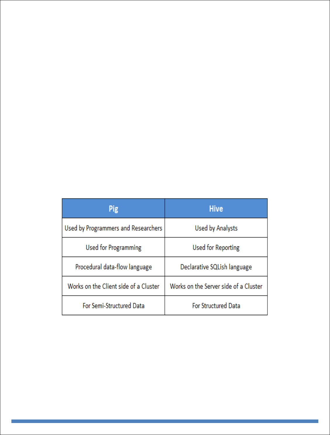
BIG DATA ANALYTICS
94
converted into a tuple. In the third statement, the words are grouped together so that the
count can be computed which is done in fourth statement.
Pig at Yahoo
Pig was initially developed by Yahoo! for its data scientists who were using Hadoop. It
was incepted to focus mainly on analysis of large datasets rather than on writing mapper
and reduce functions. This allowed users to focus on what they want to do rather than
bothering with how its done. On top of this with Pig language you have the facility to write
commands in other languages like Java, Python etc. Big applications that can be built on
Pig Latin can be custom built for different companies to serve different tasks related to data
management. Pig systemizes all the branches of data and relates it in a manner that when
the time comes, filtering and searching data is checked efficiently and quickly.
Pig Versus Hive
Pig Vs Hive
Here are some basic difference between Hive and Pig which gives an idea of which to use
depending on the type of data and purpose.
Why Go for Hive When Pig is There?
The tabular column below gives a comprehensive comparison between the two. The Hive can be
used in places where partitions are necessary and when it is essential to define and create cross-
language services for numerous languages.
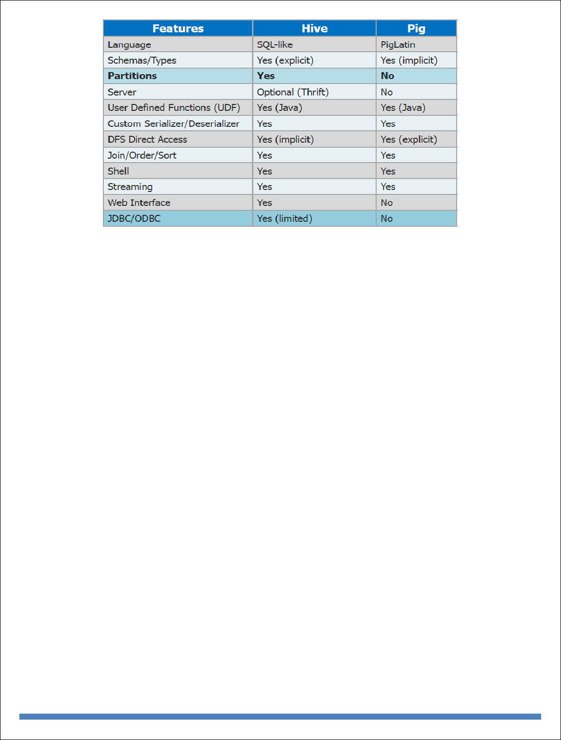
BIG DATA ANALYTICS
95

BIG DATA ANALYTICS
96
UNIT-V
Overview of machine learning (ML)
Machine learning is a branch in computer science that studies the design of algorithms that can
learn. Typical machine learning tasks are concept learning, function learning or “predictive
modeling”, clustering and finding predictive patterns. These tasks are learned through available
data that were observed through experiences or instructions, for example. Machine learning hopes
that including the experience into its tasks will eventually improve the learning. The ultimate goal
is to improve the learning in such a way that it becomes automatic, so that humans like ourselves
don’t need to interfere any more.
In supervised learning (SML), the learning algorithm is presented with labelled example
inputs, where the labels indicate the desired output. SML itself is composed of classification,
where the output is categorical, and regression, where the output is numerical.
In unsupervised learning (UML), no labels are provided, and the learning algorithm focuses
solely on detecting structure in unlabelled input data.
Note that there are also semi-supervised learning approaches that use labelled data to inform
unsupervised learning on the unlabelled data to identify and annotate new classes in the dataset
(also called novelty detection).
Reinforcement learning, the learning algorithm performs a task using feedback from operating
in a real or synthetic environment.
Broadly, there are 3 types of Machine Learning Algorithms
1. Supervised Learning
2. Unsupervised Learning
3. Reinforcement Learning:

BIG DATA ANALYTICS
97
List of Common Machine Learning Algorithms
Here is the list of commonly used machine learning algorithms. These algorithms can be applied to
almost any data problem:
1. Linear Regression
2. Logistic Regression
3. Decision Tree
4. SVM
5. Naive Bayes
6. kNN
7. K-Means
8. Random Forest
9. Dimensionality Reduction Algorithms
10. Gradient Boosting algorithms
1. GBM
2. XGBoost
3. LightGBM
4. CatBoost
Regression analysis consists of a set of machine learning methods that allow us to predict a continuous outcome
variable (y) based on the value of one or multiple predictor variables (x).
Briefly, the goal of regression model is to build a mathematical equation that defines y as a function of the x variables.
Next, this equation can be used to predict the outcome (y) on the basis of new values of the predictor variables (x).
Linear regression is the most simple and popular technique for predicting a continuous variable. It assumes a linear
relationship between the outcome and the predictor variables.
The linear regression equation can be written as y = b0 + b*x + e, where:
b0 is the intercept,
b is the regression weight or coefficient associated with the predictor variable x.
e is the residual error
Technically, the linear regression coefficients are detetermined so that the error in predicting the outcome value is
minimized. This method of computing the beta coefficients is called the Ordinary Least Squares method.
When you have multiple predictor variables, say x1 and x2, the regression equation can be written as y = b0 + b1*x1
+ b2*x2 +e. In some situations, there might be an interaction effect between some predictors, that is for example,
increasing the value of a predictor variable x1 may increase the effectiveness of the predictor x2 in explaining the
variation in the outcome variable.
Note also that, linear regression models can incorporate both continuous and categorical predictor variables.
When you build the linear regression model, you need to diagnostic whether linear model is suitable for your data.
In some cases, the relationship between the outcome and the predictor variables is not linear. In these situations, you
need to build a non-linear regression, such as polynomial and spline regression.
When you have multiple predictors in the regression model, you might want to select the best combination of predictor
variables to build an optimal predictive model. This process called model selection, consists of comparing multiple
models containing different sets of predictors in order to select the best performing model that minimize the prediction
error. Linear model selection approaches include best subsets regression and stepwise regression
In some situations, such as in genomic fields, you might have a large multivariate data set containing some correlated
predictors. In this case, the information, in the original data set, can be summarized into few new variables (called
principal components) that are a linear combination of the original variables. This few principal components can be
used to build a linear model, which might be more performant for your data. This approach is know as principal
component-based methods, which include: principal component regression and partial least squares regression.

BIG DATA ANALYTICS
98
An alternative method to simplify a large multivariate model is to use penalized regression, which penalizes the
model for having too many variables. The most well known penalized regression include ridge regression and
the lasso regression.
You can apply all these different regression models on your data, compare the models and finally select the best
approach that explains well your data. To do so, you need some statistical metrics to compare the performance of the
different models in explaining your data and in predicting the outcome of new test data.
The best model is defined as the model that has the lowest prediction error. The most popular metrics for comparing
regression models, include:
Root Mean Squared Error, which measures the model prediction error. It corresponds to the average difference
between the observed known values of the outcome and the predicted value by the model. RMSE is computed
as RMSE = mean((observeds - predicteds)^2) %>% sqrt(). The lower the RMSE, the better the model.
Adjusted R-square, representing the proportion of variation (i.e., information), in your data, explained by the
model. This corresponds to the overall quality of the model. The higher the adjusted R2, the better the model
Note that, the above mentioned metrics should be computed on a new test data that has not been used to train (i.e. build)
the model. If you have a large data set, with many records, you can randomly split the data into training set (80% for
building the predictive model) and test set or validation set (20% for evaluating the model performance).
One of the most robust and popular approach for estimating a model performance is k-fold cross-validation. It can
be applied even on a small data set. k-fold cross-validation works as follow:
1. Randomly split the data set into k-subsets (or k-fold) (for example 5 subsets)
2. Reserve one subset and train the model on all other subsets
3. Test the model on the reserved subset and record the prediction error
4. Repeat this process until each of the k subsets has served as the test set.
5. Compute the average of the k recorded errors. This is called the cross-validation error serving as the performance
metric for the model.
Clustering in Machine Learning
Clustering or cluster analysis is a machine learning technique, which groups the unlabelled dataset. It can be defined
as "A way of grouping the data points into different clusters, consisting of similar data points. The objects with the
possible similarities remain in a group that has less or no similarities with another group."
It does it by finding some similar patterns in the unlabelled dataset such as shape, size, color, behavior, etc., and
divides them as per the presence and absence of those similar patterns.
It is an unsupervised learning method, hence no supervision is provided to the algorithm, and it deals with the
unlabeled dataset.
After applying this clustering technique, each cluster or group is provided with a cluster-ID. ML system can use this
id to simplify the processing of large and complex datasets.
The clustering technique is commonly used for statistical data analysis.
Example: Let's understand the clustering technique with the real-world example of Mall: When we visit any shopping
mall, we can observe that the things with similar usage are grouped together. Such as the t-shirts are grouped in one
section, and trousers are at other sections, similarly, at vegetable sections, apples, bananas, Mangoes, etc., are grouped
in separate sections, so that we can easily find out the things. The clustering technique also works in the same way.
Other examples of clustering are grouping documents according to the topic.
The clustering technique can be widely used in various tasks. Some most common uses of this technique are:
o Market Segmentation
o Statistical data analysis
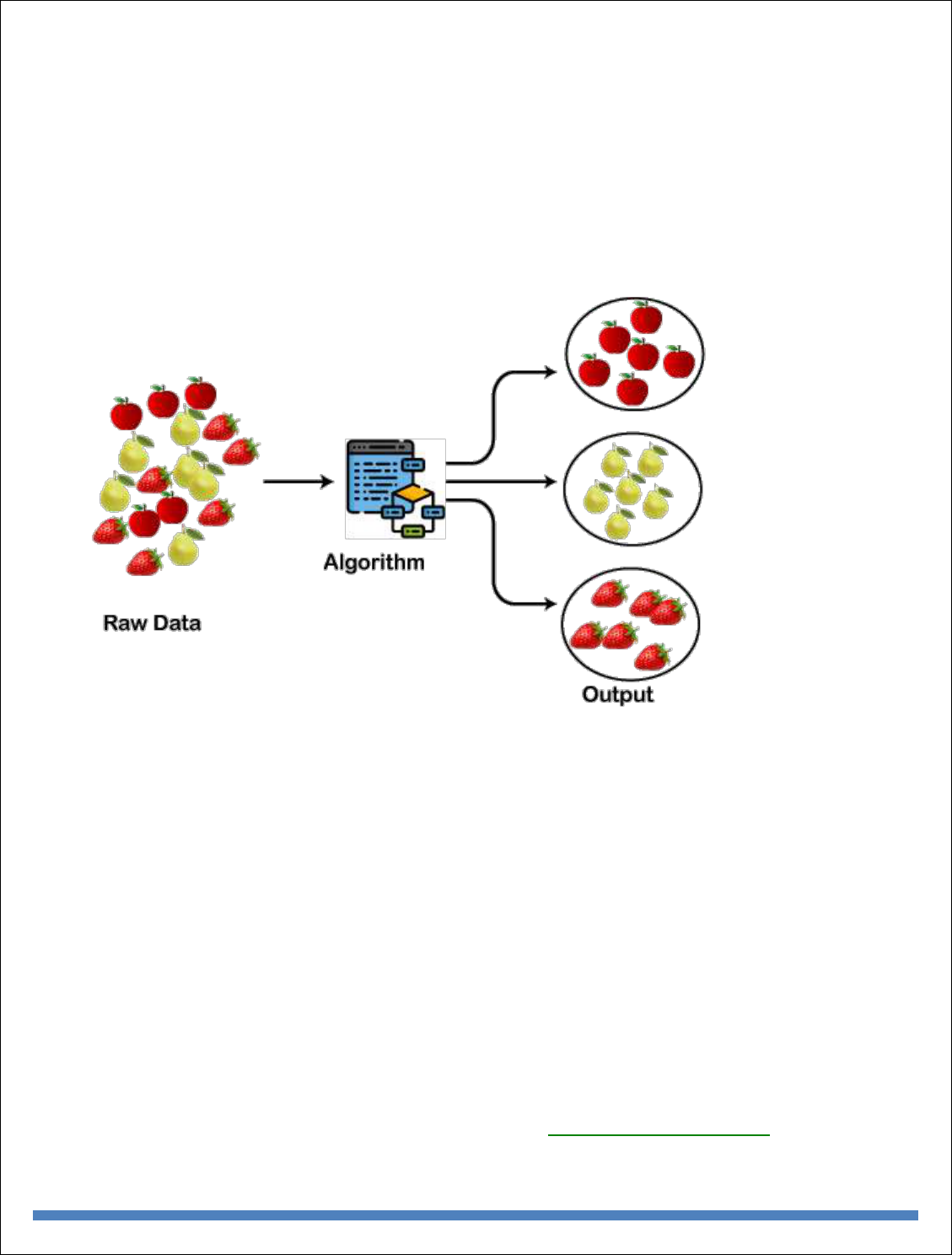
BIG DATA ANALYTICS
99
o Social network analysis
o Image segmentation
o Anomaly detection, etc.
Apart from these general usages, it is used by the Amazon in its recommendation system to provide the
recommendations as per the past search of products. Netflix also uses this technique to recommend the movies and
web-series to its users as per the watch history.
The below diagram explains the working of the clustering algorithm. We can see the different fruits are divided into
several groups with similar properties.
Types of Clustering Methods
The clustering methods are broadly divided into Hard clustering (datapoint belongs to only one group) and Soft
Clustering (data points can belong to another group also). But there are also other various approaches of Clustering
exist. Below are the main clustering methods used in Machine learning:
1. Partitioning Clustering
2. Density-Based Clustering
3. Distribution Model-Based Clustering
4. Hierarchical Clustering
5. Fuzzy Clustering
Partitioning Clustering
It is a type of clustering that divides the data into non-hierarchical groups. It is also known as the centroid-based
method. The most common example of partitioning clustering is the K-Means Clustering algorithm.
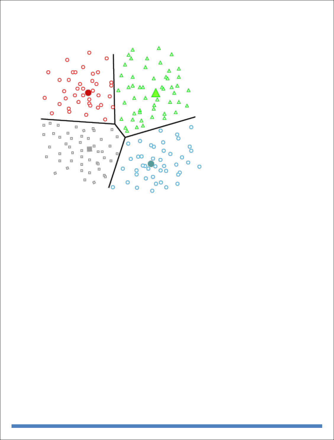
BIG DATA ANALYTICS
100
In this type, the dataset is divided into a set of k groups, where K is used to define the number of pre-defined groups.
The cluster center is created in such a way that the distance between the data points of one cluster is minimum as
compared to another cluster centroid.
Density-Based Clustering
The density-based clustering method connects the highly-dense areas into clusters, and the arbitrarily shaped
distributions are formed as long as the dense region can be connected. This algorithm does it by identifying different
clusters in the dataset and connects the areas of high densities into clusters. The dense areas in data space are divided
from each other by sparser areas.
These algorithms can face difficulty in clustering the data points if the dataset has varying densities and high
dimensions.
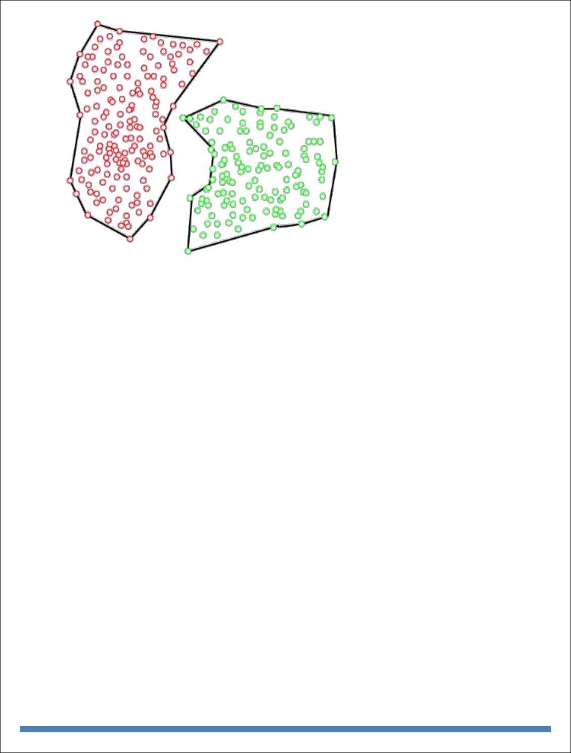
BIG DATA ANALYTICS
101
Distribution Model-Based Clustering
In the distribution model-based clustering method, the data is divided based on the probability of how a dataset belongs
to a particular distribution. The grouping is done by assuming some distributions commonly Gaussian Distribution.
The example of this type is the Expectation-Maximization Clustering algorithm that uses Gaussian Mixture Models
(GMM).
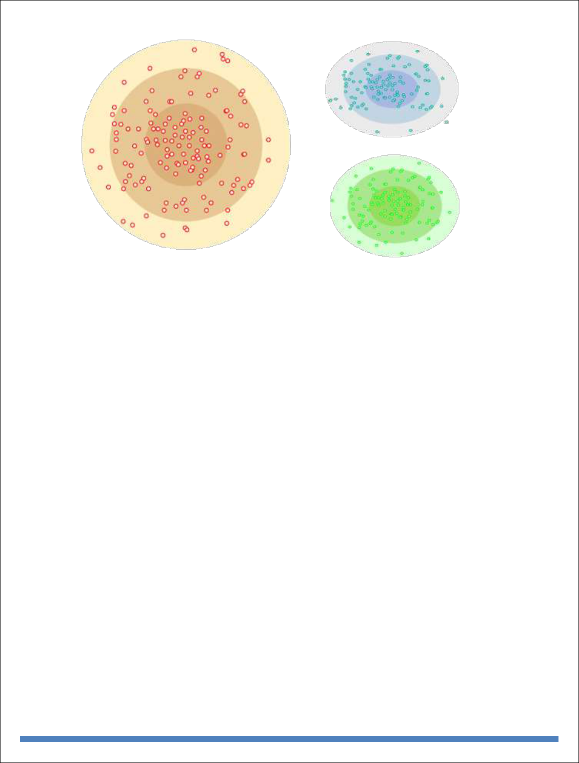
BIG DATA ANALYTICS
102
Fuzzy Clustering
Fuzzy clustering is a type of soft method in which a data object may belong to more than one group or cluster. Each
dataset has a set of membership coefficients, which depend on the degree of membership to be in a cluster. Fuzzy C-
means algorithm is the example of this type of clustering; it is sometimes also known as the Fuzzy k-means algorithm.
Clustering Algorithms
The Clustering algorithms can be divided based on their models that are explained above. There are different types of
clustering algorithms published, but only a few are commonly used. The clustering algorithm is based on the kind of
data that we are using. Such as, some algorithms need to guess the number of clusters in the given dataset, whereas
some are required to find the minimum distance between the observation of the dataset.
Here we are discussing mainly popular Clustering algorithms that are widely used in machine learning:
1. K-Means algorithm: The k-means algorithm is one of the most popular clustering algorithms. It classifies
the dataset by dividing the samples into different clusters of equal variances. The number of clusters must be
specified in this algorithm. It is fast with fewer computations required, with the linear complexity of O(n).
2. Mean-shift algorithm: Mean-shift algorithm tries to find the dense areas in the smooth density of data
points. It is an example of a centroid-based model, that works on updating the candidates for centroid to be
the center of the points within a given region.
3. DBSCAN Algorithm: It stands for Density-Based Spatial Clustering of Applications with Noise. It is an
example of a density-based model similar to the mean-shift, but with some remarkable advantages. In this
algorithm, the areas of high density are separated by the areas of low density. Because of this, the clusters
can be found in any arbitrary shape.

BIG DATA ANALYTICS
103
4. Expectation-Maximization Clustering using GMM: This algorithm can be used as an alternative for the
k-means algorithm or for those cases where K-means can be failed. In GMM, it is assumed that the data
points are Gaussian distributed.
5. Agglomerative Hierarchical algorithm: The Agglomerative hierarchical algorithm performs the bottom-
up hierarchical clustering. In this, each data point is treated as a single cluster at the outset and then
successively merged. The cluster hierarchy can be represented as a tree-structure.
6. Affinity Propagation: It is different from other clustering algorithms as it does not require to specify the
number of clusters. In this, each data point sends a message between the pair of data points until convergence.
It has O(N
2
T) time complexity, which is the main drawback of this algorithm.
Applications of Clustering
Below are some commonly known applications of clustering technique in Machine Learning:
o In Identification of Cancer Cells: The clustering algorithms are widely used for the identification of
cancerous cells. It divides the cancerous and non-cancerous data sets into different groups.
o In Search Engines: Search engines also work on the clustering technique. The search result appears based
on the closest object to the search query. It does it by grouping similar data objects in one group that is far
from the other dissimilar objects. The accurate result of a query depends on the quality of the clustering
algorithm used.
o Customer Segmentation: It is used in market research to segment the customers based on their choice and
preferences.
o In Biology: It is used in the biology stream to classify different species of plants and animals using the image
recognition technique.
o In Land Use: The clustering technique is used in identifying the area of similar lands use in the GIS database.
This can be very useful to find that for what purpose the particular land should be used, that means for which
purpose it is more suitable.
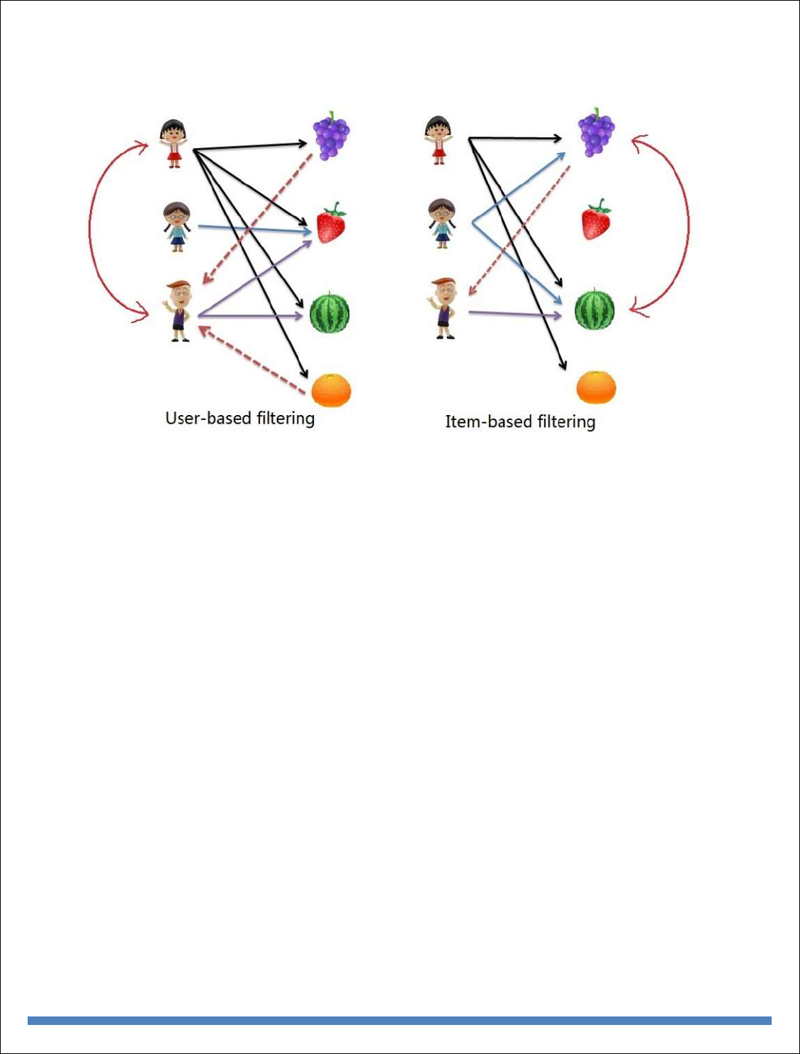
BIG DATA ANALYTICS
104
Collaborative Filtering with R
Collaborative filtering is another technique that can be used for recommendation.
The underlying concept behind this technique is as follows:
Assume Person A likes Oranges, and Person B likes Oranges.
Assume Person A likes Apples.
Person B is likely to have similar opinions on Apples as A than some other random person.
The implications of collaborative filtering are obvious: you can predict and recommend items to
users based on preference similarities. There are two types of collaborative filtering: user-based
and item-based.
Item Based Collaborative Filtering takes the similarities between items’ consumption history.
User Based Collaborative Filtering considers similarities between user consumption history.
Association Rule Mining
Association Rule Mining is used when you want to find an association between different objects
in a set, find frequent patterns in a transaction database, relational databases or any other
information repository. The applications of Association Rule Mining are found in Marketing,
Basket Data Analysis (or Market Basket Analysis) in retailing, clustering and classification. It can
tell you what items do customers frequently buy together by generating a set of rules
BIG DATA ANALYTICS
105
called Association Rules. In simple words, it gives you output as rules in form if this then that.
Clients can use those rules for numerous marketing strategies:
Changing the store layout according to trends
Customer behavior analysis
Catalogue design
Cross marketing on online stores
What are the trending items customers buy
Customized emails with add-on sales
Consider the following example:
Given is a set of transaction data. You can see transactions numbered 1 to 5. Each
transaction shows items bought in that transaction. You can see that Diaper is bought with Beer in

BIG DATA ANALYTICS
106
three transactions. Similarly, Bread is bought with milk in three transactions making them both
frequent item sets. Association rules are given in the form as below:
A=>B[Support,Confidence]A=>B[Support,Confidence]
The part before =>=> is referred to as if (Antecedent) and the part after =>=> is referred to as then
(Consequent).
Where A and B are sets of items in the transaction data. A and B are disjoint sets.
Computer=>Anti−virusSoftware[Support=20%,confidence=60%]Computer=>Anti−virusSoftwar
e[Support=20%,confidence=60%]
Above rule says:
1. 20% transaction show Anti-virus software is bought with purchase of a Computer
2. 60% of customers who purchase Anti-virus software is bought with purchase of a
Computer
In the following section you will learn about the basic concepts of Association Rule Mining:
Basic Concepts of Association Rule Mining
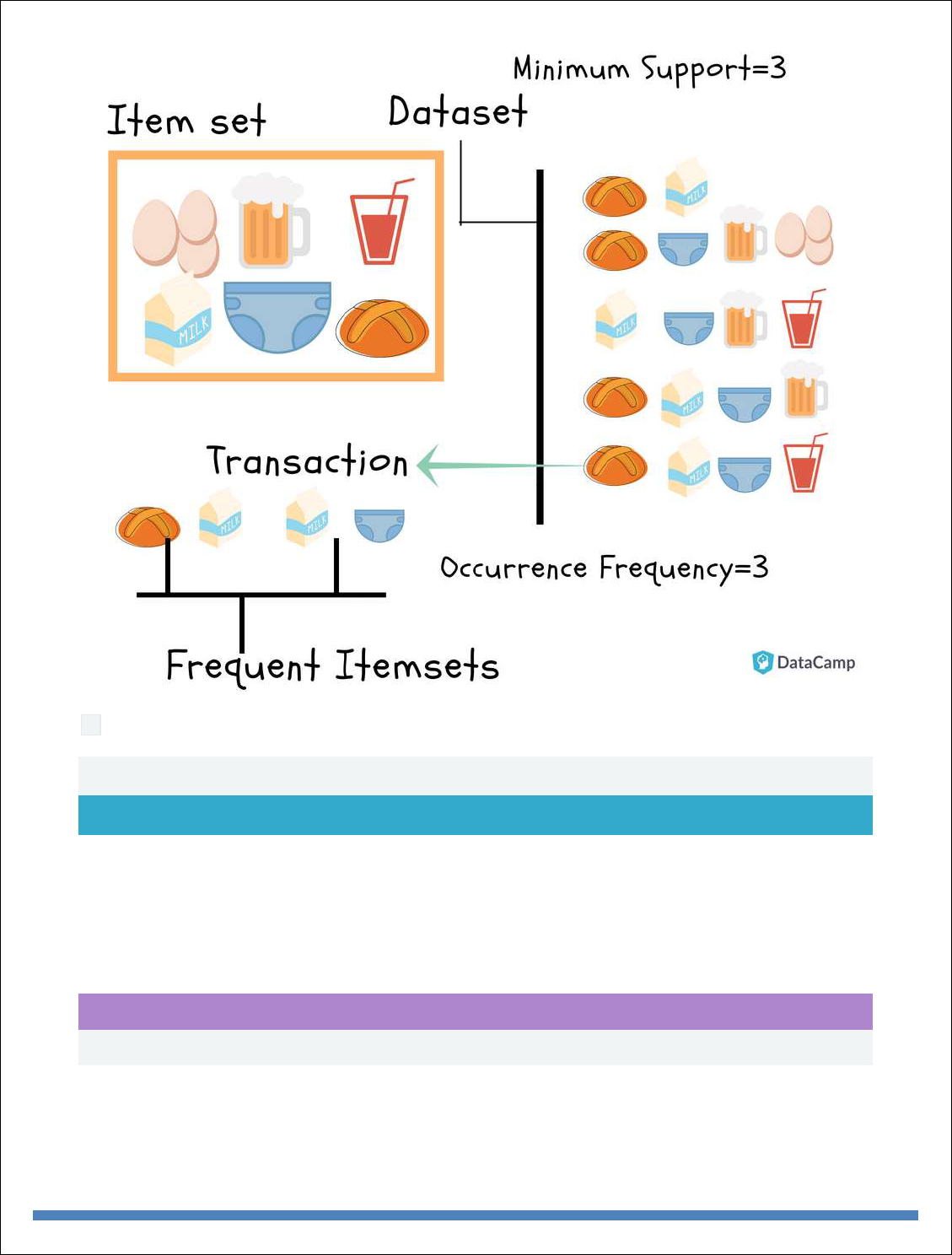

BIG DATA ANALYTICS
108
Market Basket Analysis using R
Learn about Market Basket Analysis & the APRIORI Algorithm that works behind it. You'll see
how it is helping retailers boost business by predicting what items customers buy together.
You are a data scientist (or becoming one!), and you get a client who runs a retail store. Your client
gives you data for all transactions that consists of items bought in the store by several customers
over a period of time and asks you to use that data to help boost their business. Your client will
use your findings to not only change/update/add items in inventory but also use them to change
the layout of the physical store or rather an online store. To find results that will help your client,
you will use Market Basket Analysis (MBA) which uses Association Rule Mining on the given
transaction data.
Association Rule Mining
Association Rule Mining is used when you want to find an association between different objects
in a set, find frequent patterns in a transaction database, relational databases or any other
information repository. The applications of Association Rule Mining are found in Marketing,
Basket Data Analysis (or Market Basket Analysis) in retailing, clustering and classification. It can
tell you what items do customers frequently buy together by generating a set of rules
called Association Rules. In simple words, it gives you output as rules in form if this then that.
Clients can use those rules for numerous marketing strategies:
Changing the store layout according to trends
Customer behavior analysis
Catalogue design
Cross marketing on online stores
What are the trending items customers buy
Customized emails with add-on sales
BIG DATA ANALYTICS
109
Consider the following example:
Given is a set of transaction data. You can see transactions numbered 1 to 5. Each transaction
shows items bought in that transaction. You can see that Diaper is bought with Beer in three
transactions. Similarly, Bread is bought with milk in three transactions making them both frequent
item sets. Association rules are given in the form as below:
A=>B[Support,Confidence]A=>B[Support,Confidence]
The part before =>=> is referred to as if (Antecedent) and the part after =>=> is referred to as then
(Consequent).
Where A and B are sets of items in the transaction data. A and B are disjoint sets.
Computer=>Anti−virusSoftware[Support=20%,confidence=60%]Computer=>Anti−virusSoftwar
e[Support=20%,confidence=60%]
Above rule says:
1. 20% transaction show Anti-virus software is bought with purchase of a Computer
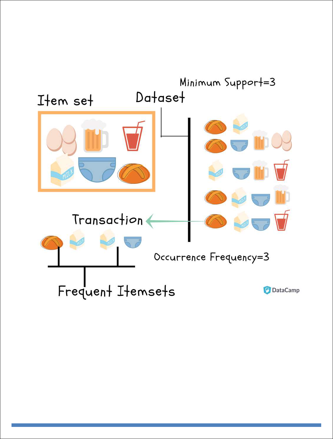
BIG DATA ANALYTICS
110
2. 60% of customers who purchase Anti-virus software is bought with purchase of a
Computer
In the following section you will learn about the basic concepts of Association Rule Mining:
Basic Concepts of Association Rule Mining
1. Itemset: Collection of one or more items. K-item-set means a set of k items.
2. Support Count: Frequency of occurrence of an item-set
3. Support (s): Fraction of transactions that contain the item-set 'X'
Support(X)=frequency(X)NSupport(X)=frequency(X)N
For a Rule A=>B, Support is given by:
Support(A=>B)=frequency(A,B)NSupport(A=>B)=frequency(A,B)N

BIG DATA ANALYTICS
111
Note: P(AUB) is the probability of A and B occurring together. P denotes probability.
Go ahead, try finding the support for Milk=>Diaper as an exercise.
1. Confidence (c): For a rule A=>B Confidence shows the percentage in which B is bought
with A.
Confidence(A=>B)=P(A∩B)P(A)=frequency(A,B)frequency(A)Confidence(A=>B)=P(A∩B)P(
A)=frequency(A,B)frequency(A)
The number of transactions with both A and B divided by the total number of transactions having
A.
Confidence(Bread=>Milk)=34=0.75=75%Confidence(Bread=>Milk)=34=0.75=75%
Now find the confidence for Milk=>Diaper.
Note: Support and Confidence measure how interesting the rule is. It is set by the minimum
support and minimum confidence thresholds. These thresholds set by client help to compare the
rule strength according to your own or client's will. The closer to threshold the more the rule is of
use to the client.
1. Frequent Itemsets: Item-sets whose support is greater or equal than minimum support
threshold (min_sup). In above example min_sup=3. This is set on user choice.
2. Strong rules: If a rule A=>B[Support, Confidence] satisfies min_sup and min_confidence
then it is a strong rule.
3. Lift: Lift gives the correlation between A and B in the rule A=>B. Correlation shows how
one item-set A effects the item-set B.
Lift(A=>B)=SupportSupp(A)Supp(B)Lift(A=>B)=SupportSupp(A)Supp(B)
For example, the rule {Bread}=>{Milk}, lift is calculated as:
support(Bread)=45=0.8support(Bread)=45=0.8
support(Milk)=45=0.8support(Milk)=45=0.8

BIG DATA ANALYTICS
112
Lift(Bread=>Milk)=0.60.8∗0.8=0.9Lift(Bread=>Milk)=0.60.8∗0.8=0.9
If the rule had a lift of 1,then A and B are independent and no rule can be derived from
them.
If the lift is > 1, then A and B are dependent on each other, and the degree of which is given
by ift value.
If the lift is < 1, then presence of A will have negative effect on B.
Goal of Association Rule Mining
When you apply Association Rule Mining on a given set of transactions T your goal will be to find
all rules with:
1. Support greater than or equal to min_support
2. Confidence greater than or equal to min_confidence
APRIORI Algorithm
In this part of the tutorial, you will learn about the algorithm that will be running
behind R libraries for Market Basket Analysis. This will help you understand your
clients more and perform analysis with more attention. If you already know about
the APRIORI algorithm and how it works, you can get to the coding part.
Association Rule Mining is viewed as a two-step approach:
1. Frequent Itemset Generation: Find all frequent item-sets with support >=
pre-determined min_support count
2. Rule Generation: List all Association Rules from frequent item-sets.
Calculate Support and Confidence for all rules. Prune rules that fail
min_support and min_confidence thresholds.
Frequent Itemset Generation is the most computationally expensive step because
it requires a full database scan.
Among the above steps, Frequent Item-set generation is the most costly in terms of computation.
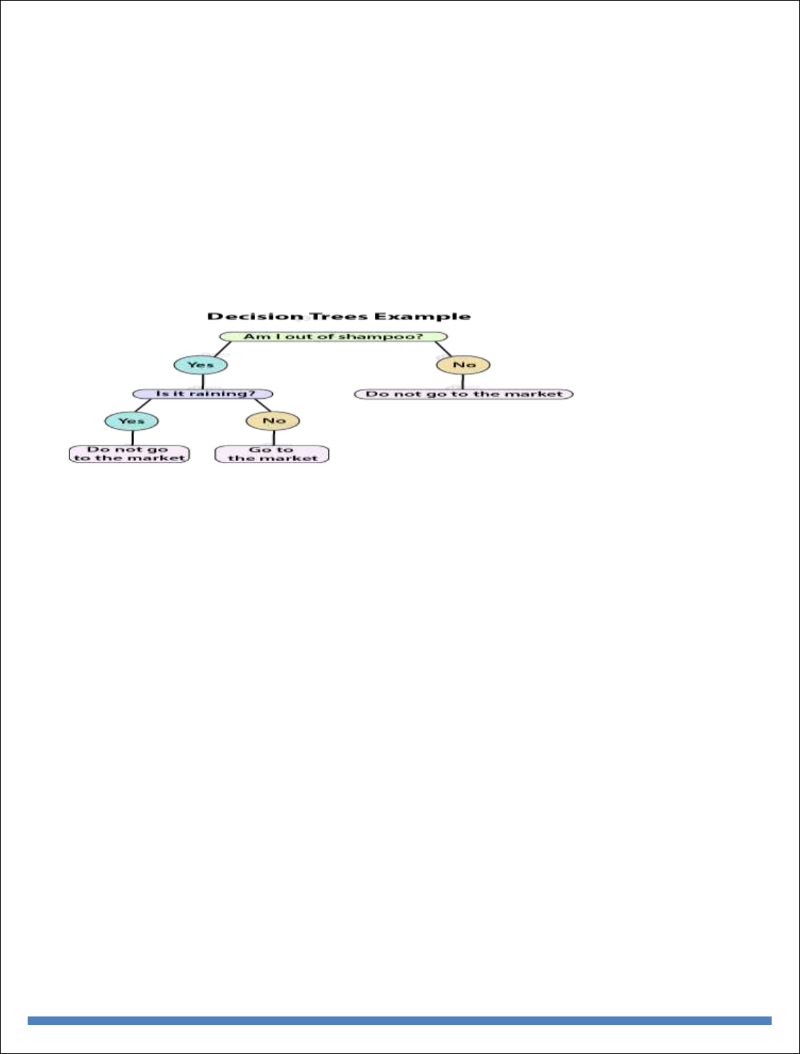
BIG DATA ANALYTICS
113
Above you have seen the example of only 5 transactions, but in real-world transaction data for
retail can exceed up to GB s and TBs of data for which an optimized algorithm is needed to prune
out Item-sets that will not help in later steps. For this APRIORI Algorithm is used.
Decision Trees
Decision Trees are a popular Data Mining technique that makes use of a tree-like structure to
deliver consequences based on input decisions. One important property of decision trees is that it
is used for both regression and classification. This type of classification method is capable of
handling heterogeneous as well as missing data. Decision Trees are further capable of producing
understandable rules. Furthermore, classifications can be performed without many computations.
As mentioned above, both the classification and regression tasks can be performed with the help
of Decision Trees. You can perform either classification or regression tasks here. Decision Trees
can be visualised as follows:
To create a decision tree, you need to follow certain steps:
1. Choosing a Variable
2. Assigning Data to Nodes
3. Pruning the Tree
Common R Decision Trees Algorithms
There are three most common Decision Tree Algorithms:
Classification and Regression Tree (CART) investigates all kinds of variables.
Zero (developed by J.R. Quinlan) works by aiming to maximize information gain achieved
by assigning each individual to a branch of the tree.
Chi-Square Automation Interaction Detection (CHAID) – It is reserved for the
investigation of discrete and qualitative independent and dependent variabl
Applications of Decision Trees
Decision Trees are used in the following areas of applications:
Marketing and Sales – Decision Trees play an important role in a decision-oriented sector
like marketing. In order to understand the consequences of marketing activities, organisations

BIG DATA ANALYTICS
114
make use of Decision Trees to initiate careful measures. This helps in making efficient
decisions that help the company to reap profits and minimize losses.
Reducing Churn Rate – Banks make use of machine learning algorithms like Decision
Trees to retain their customers. It is always cheaper to keep customers than to gain new ones.
Banks are able to analyze which customers are more vulnerable to leaving their business.
Based on the output, they are able to make decisions by providing better services, discounts
as well as several other features. This ultimately helps them to reduce the churn rate.
Anomaly & Fraud Detection – Industries like finance and banking suffer from various cases
of fraud. In order to filter out anomalous or fraud loan applications, information and insurance
fraud, these companies deploy decision trees to provide them with the necessary information
to identify fraudulent customers.
Medical Diagnosis – Classification trees identifies patients who are at risk of suffering from
serious diseases such as cancer and diabetes.
How to Create Decision Trees in R
The Decision Tree techniques can detect criteria for the division of individual items of a group
into predetermined classes that are denoted by n.
In the first step, the variable of the root node is taken. This variable should be selected based on
its ability to separate the classes efficiently. This operation starts with the division of variable into
the given classes. This results in the creation of subpopulations. This operation repeats until no
separation can be obtained.
A tree exhibiting not more than two child nodes is a binary tree. The origin node is referred to as
a node and the terminal nodes are the trees.
Defining Big Data
Big data is not a single technology but a combination of old and new technologies that helps
companies gain actionable insight. Therefore, big data is the capability to manage a huge volume
of disparate data, at the right speed, and within the right time frame to allow real-time analysis and
reaction. As we note earlier in this chapter, big data is typically broken down by three
characteristics: ✓ Volume: How much data ✓ Velocity: How fast that data is processed ✓ Variety:
The various types of data Although it’s convenient to simplify big data into the three Vs, it can be
misleading and overly simplistic. For example, you may be managing a relatively small amount
of very disparate, complex data or you may be processing a huge volume of very simple data. That
simple data may be all structured or all unstructured. Even more important is the fourth V: veracity.
How accurate is that data in predicting business value? Do the results of a big data analysis actually
make sense? It is critical that you don’t underestimate the task at hand. Data must be able to be
verified based on both accuracy and context. An innovative business may want to be able to
analyze massive amounts of data in real time to quickly assess the value of that customer and the
potential to provide additional offers to that customer. It is necessary to identify the right amount
and types of data that can be analyzed to impact business outcomes. Big data incorporates all data,
including structured data and unstructured data from e-mail, social media, text streams, and more.
This kind of data management requires that companies leverage both their structured and
unstructured data
Installing R packages
To use the data file with the format specified earlier, we don't need to install extra R packages. We
just need to use the built-in functions available with R. Importing the data into R To perform

BIG DATA ANALYTICS
115
analytics-related activities, we need to use the following functions to get the data into R: • CSV:
read.csv() is intended for reading the comma separated value (CSV) files, where the decimal point
is ",".
The retrieved data will be stored into one R object, which is considered as Dataframe. Dataframe
<- read.csv("data.csv",sep=",") • TXT: To retrieve the tab separated values, the read.table()
function will be used with some important parameters and the return type of this function will be
Dataframe type. Dataframe <- read.table("data.csv", sep="\t") • .RDATA: Here, the .
RDATA format is used by R for storing the workspace data for a particular time period. It is
considered as image file. This will store/retrieve all of the data available in the workspace.
load("history.RDATA") • .rda: This is also R's native data format, which stores the specific data
variable as per requirement. load("data_variables_a_and_b.rda")
Exporting the data from R To export the existing data object from R and to support data files as
per requirements, we need to use the following functions: • CSV: Write the dataframe object into
the csv data file via the following command: write.csv(mydata, "c:/mydata.csv", sep=",",
row.names=FALSE) •
TXT: Write the data with the tab delimiters via the following command: write.table(mydata,
"c:/mydata.txt", sep="\t") • .RDATA: To store the workspace data variables available to R session,
use the following command: save.image() • .rda: This function is used to store specific data objects
that can be reused later. Use the following code for saving them to the .rda files. # column vector
a <- c(1,2,3) # column vector b <- c(2,4,6) # saving it to R (.rda) data format save(a, b, file="
data_variables_a_and_b.rda")
Importing the data into R We know how to check MySQL tables and their fields. After
identification of useful data tables, we can import them in R using the following RMySQL
command.
To retrieve the custom data from MySQL database as per the provided SQL query, we need to
store it in an object: rs = dbSendQuery(mydb, "select * from sample_table") The available data-
related information can be retrieved from MySQL to R via the fetch command as follows: dataset
= fetch(rs, n=-1) Here, the specified parameter n = -1 is used for retrieving all pending records.
